Next: Kernel Basis Functions
Up: svkde
Previous: Non-Parametric Density Estimation
In the previous section we decomposed the CDF into regions or windows
 and estimated the PDF for each window separately. There are several ways to choose the placement (i.e. the center) of the windows; for example they can be disjoint and cover the entire domain as is the case with Frequency Histogram Estimation (Figure 2); the benefit of using such a method is that the structure of the windows are independant of the number of random samples (although the estimation procedure is not). Alternatively, the approach we will consider henceforth will associate a window with each random sample
  so that we have a sequence of windows
 centered at
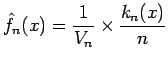
 . Since the number of windows (and their volume) is now dependent on the sample size we will re-write the result (5) as
 |
(6) |
where  is the volume of the region
 and
and  is the number of samples that fall inside it; as more samples are generated the regions can either be refined (as is the case with the Parzen method) or we can reverse this logic and gradually increase the size of the regions starting with an inconspicuously small
 (which is the case with the nearest-neighbor estimation method).
Let us further generalize [DHS01] the definition of the region
so that we can estimate multi-variate densities; assume the windows
are d-dimensional hypercubes with edges of length  ; the volume is then simply
 .
.
Figure:
Let the hypercube window
have dimension  ; then
  is simply a count of the random samples that fall in the square with sides of length and centered at
  ; in this case
  .
.
|
|
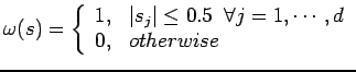
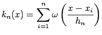
Now that the window has changed we need to revise our definition of which was previously defined using a simple indicator function
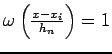
 ; generalising this from counting random samples within an interval to counting within a hypercube can be done by first using a window function
  of the form:
which defines the boundary for a unit-hypercube centered at the origin and then defining as follows:
So
of the form:
which defines the boundary for a unit-hypercube centered at the origin and then defining as follows:
So
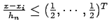
 if and only if
 or
or
 , in other words if is less than half the length of an edge of the hypercube away from in all dimensions
 . So
. So
 defines a (d+1)-dimensional hypercube of volume
  (since the (d+1)th dimension has edges of length
  ), centered at which counts the number of random samples that fall within the d-dimensional hypercube window
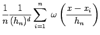
. Finally substituting this result into 6 gives:
), centered at which counts the number of random samples that fall within the d-dimensional hypercube window
. Finally substituting this result into 6 gives:
The resulting estimated density is `jagged' since the window (basis) functions in the above linear combination are hypercubes (Figure 3) with abrupt edges; reducing the width as more samples are generated will smooth out the estimate. Infact if
 then the estimated density function is proved [Fuk72] to be asymptotically unbiased;
 .
.
Subsections
Next: Kernel Basis Functions
Up: svkde
Previous: Non-Parametric Density Estimation
Rohan Shiloh SHAH
2006-12-12
![\includegraphics[scale=1.25]{image_hypercube_window_function.eps}](img86.png)