Next: Kernel Density Estimation: Parzen
Up: svkde
Previous: svkde
Provided with  discrete observations of a random variable
all of which are identically and independently distributed (iid) according to some unknown probability distribution
discrete observations of a random variable
all of which are identically and independently distributed (iid) according to some unknown probability distribution  , we seek an estimate
 of the true probability density function
  . The search for
is usually performed in a restricted functional space
. The search for
is usually performed in a restricted functional space
 ; which is infact a Reproducing Kernel Hilbert Space (see Section
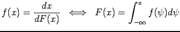
 ![[*]](file:/usr/local/share/latex2html/icons/crossref.png) ). The functional space is further restricted to only those functions that are non-negative and integrate to one. The probability density function (PDF) is simply the derivative of the cumulative distribution function (CDF):
). The functional space is further restricted to only those functions that are non-negative and integrate to one. The probability density function (PDF) is simply the derivative of the cumulative distribution function (CDF):
 |
(2) |
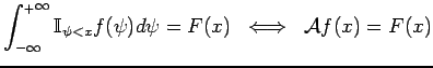
We can rewrite 2 as a linear mapping [WGS+99]:
 |
(3) |
where both integrals in 2 and 3 are vector integrations and
 is an injective mapping from
to the Hilbert Space where
is an injective mapping from
to the Hilbert Space where  is defined;
 . Neither
  or are known (whereas the operator
and its inverse are well defined) so we begin by estimating using samples
or are known (whereas the operator
and its inverse are well defined) so we begin by estimating using samples
 generated by the random process and then proceed to deriving
  from our estimate
  using an approximation of the inverse of the linear transformation
.
using an approximation of the inverse of the linear transformation
.
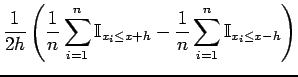
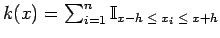
The empirical distribution at  can be estimated from the data by taking the ratio of the number of samples that are less than or equal to to the total number of samples:
![$\displaystyle \hat{F}(x) = \frac{1}{n}\sum_{i=1}^n \mathbb{I}_{( -\infty, \; x_i]} (x)$](img45.png) |
(4) |
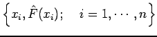
and is an unbiased maximum likelihood estimate that is piece-wise constant. For the density to exist, the estimated distribution must be differentiable and hence continuous and so to smooth out the estimate ; a non-linear regression (Figure 1) is used to approximate the distribution in the regions where training samples are unavailable; specifically the regression is performed on the set of pairs
and is parametrized by the vector  which leads to our new estimate for the distribution:
 . Support Vector Regression techniques may also be used to derive accurate regressions since regularization (see Section ) is then possible.
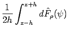
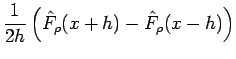
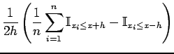
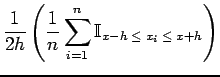
Now to estimate the density function at we need to estimate the derivative of
which can roughly be done by taking the difference between two evaluations of the distribution function at fixed lengths  and
and  from :
Figure:
Estimating the Density and Distribution Functions: [left] A linear interpolation on
 between the end points of the region
![$ \mathcal{R}= [x-h, x+h]$](img52.png) gives us an estimate for the slope
. [right] A non-linear regression on evaluations of 4 at all training samples, in this case on
gives us an estimate for the slope
. [right] A non-linear regression on evaluations of 4 at all training samples, in this case on
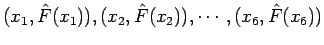 , yields a smooth estimate for the distribution function.
![\includegraphics[scale=1]{image_density_interpolation.eps}](img54.png) |
Figure 2:
Parametric Frequency Histogram Estimation: The true unknown density (top left) can be estimated by taking random samples (top right, 1000 random samples) and placing them in bins of fixed length to generate a histogram. Histograms with bin-size  ,
,  ,
,  and
and  are shown; the bin-size or bandwidth (as well as the actual placement of the bins) is an important parameter in estimating the density function; in this case only a bin-size of is able to capture the multi-modality of the true density. In the limit as the bandwidth goes to zero the histogram will converge to the true density provided the number of samples goes to infinity.
![\includegraphics[scale=0.5]{image_histogram_original_curve_01.eps}](img55.png)
![\includegraphics[scale=0.5]{image_histogram_random_samples_01.eps}](img56.png)
![\includegraphics[scale=0.5]{image_histogram_02_01.eps}](img57.png)
![\includegraphics[scale=0.5]{image_histogram_01_01.eps}](img58.png)
![\includegraphics[scale=0.5]{image_histogram_001_01.eps}](img59.png)
![\includegraphics[scale=0.5]{image_histogram_0001_01.eps}](img60.png) |
where
 is the number of samples that fall in the region
and
is the number of samples that fall in the region
and  is the volume of
 which in this case is simply
  .
.
The shape of the region
and hence its volume can be adjusted as more random samples become availible; it has been shown [DHS01] that as the regions
get smaller (
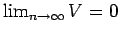 ) and the samples in the region increases (
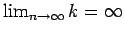 ), the estimated density
will converge to provided that
), the estimated density
will converge to provided that
 (that is to say the proportion of samples falling within the region to those outside it is very small); in the limit it will be a smooth density function.
Next: Kernel Density Estimation: Parzen
Up: svkde
Previous: svkde
Rohan Shiloh SHAH
2006-12-12