Kernel Basis Functions

Figure 4: Product Kernel Window Functions: instead of counting the number of random samples within a hypercube centered at $x$, we can associate a single-variate kernel function with each dimension and weight the count for each random sample by the product of its kernelized distances from $x$ in each dimension. More generally a multi-variate kernel function may be used.

Instead of simply counting the number of random samples that fall within a fixed volume surronding $x$, we can weight the count [DHS01] for each random sample by its kernelised distance from $x$. This can be achieved by replacing the unit hypercube window function $\omega(s)$ with a smooth, symmetric kernel density function $K(s)$ satisfying $V_n = \int_{-\infty}^{+\infty} K(s) \; ds = 1$ and $K(s) \geq 0$ and then rewriting 7 as:

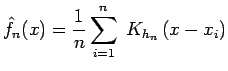$$\hat{f}_n(x) = \frac{1}{n} \sum_{i=1}^n \; K_{h_n} \left( x - x_i \right)$$ (8)

where the bandwidth $h_n$ is shifted into the definition of the kernel as the standard-deviation so that $K_{h_n}(s) = K(s/h_n)$ and the term involving the volume disappears since $V_n=1$. The gaussian kernel is most often used;

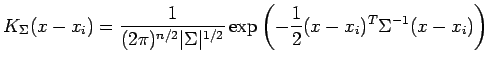$$K_\Sigma(x-x_i) = \frac{1}{(2 \pi)^{n/2} \vert \Sigma \vert^{1/2}} \exp \left( - \frac{1}{2} (x - x_i)^T \Sigma^{-1} (x - x_i) \right)$$ (9)

where $\Sigma$ is the covariance or bandwidth matrix. The key difference between the parametric density estimate 1 and non-parametric kernel density estimation 8 is that in the former the models that define the mixture have means or centers that are estimated from the data, while the latter makes use of kernel functions that are centered at the various samples in the training data.

The use of kernel basis functions has several advantages, the most significant of which is that the resulting estimate $\hat{f}(x)$ is also a smooth density function. It has been shown [Fuk72] that provided that $\lim_{n \to \infty} h_n = 0$ and $lim_{n \to \infty} n h_n = \infty$ the estimated kernel density estimate pointwise converges in probability to the true density - this is asymptotic consistency; uniform convergence in probability is also proved under the additional condition $\lim_{n \to \infty} n(h(n))^2 = \infty$.

Figure 5: Comparing the Gaussian and Epanetchnikov Kernels [Ihl03]: a bandwidth of $0.0215$ is used - the entropy for the Gaussian and Epanetchnikov Kernels are $0.0439$ and $0.0430$ respectively. Notice how even though the original or true density is defined only on the interval $[0,1]$ so that random samples are also only generated on this interval, the resulting estimated density extends outside this interval; this can be good if there are regions of missing values so that an implicit non-linear interpolation estimates the density in these regions; it can be bad when the estimation extends into regions for which the density is meant to be undefined.