The package inference contains modules that implement different inference methods as well as helper modules:
inference.engine handles the interaction between the submodules, configures the inference engine (e.g. specifies the inference algo)
inference.query specifies a query language
The inference engine handles inference.
There are different algorithms that will need to perform inference:
At this point, only one ground Bayesian network exists, GBN. If posterior samples are collected from multiple chains, e.g. in the case of MCMC inference, it would be ideal to run these chains in paralell. However this would require multiple instantiations of the ground Bayesian network. Not just the values of the vertices are required, since the network stucture changes with reference uncertainty, the whole network needs to be duplicated.
We could envision a dict() of ground Bayesian networks. Note that copy.deepcopy() doesn’t work as it would also copy all other istances, e.g. Attribute objects.
For now, changes are run sequentially and the convergence diagnostics are run on the collected samples of the posterior.
Loads the set of children attribute objects for all dependencies for the given GBN vertices of the same attribute class. The BGN is updated and potential new latent variables are added to the queue.
| Parameters: |
|---|
An uncertain relationship of type n:k has a n-side and a k-side. A ReferenceVertex is instantiated for an attribute object of the n-side and it is allowd to connect to k k-side attribute objects (which were added to the GBN by initReferenceUncertainty()).
| Parameters: | refGbnV – ReferenceVertex instance |
|---|
Loads the set of parent attribute objects for all dependencies for the given GBN vertices of the same attribute class. The BGN is updated and potential new latent variables are added to the queue.
| Parameters: |
|---|
The algorithm used for the approximate inference (e.g. gibbs,:mod:.mh )
When a uncertain relationship is first encountered, all the attribute objects that could be associated with the object that initiated the reference have to be loaded. Additionally, all the parent attributes of the exist attributes need to be loaded as well.
| Parameters: | dep – UncertainDependency instance |
|---|
The unrolled Ground Bayesian Network is a subgraph of the full graph that d-seperated the event variables Y from the query from the rest of the graph given the evidence variables.
Note
Add proper description of algorithm
Validating the GBN is necessary as there might be missing data (either because there is no datapoint or the datapoint is missing from the dataset). The standard approach would be to use an EM algorithm to find the MLE for the missing data. In order for the inference method to work we need to have valid probability distributions. In case there is a GBN vertex that has no parent vertex but a probability distribution conditional on that parent attribute, one way to avoid invalid GBN structures is to add a sampling vertex. This is only possible (and reasonable) in case this sampling vertex does not depend on parent values it
When making inference in a PRM, specifying a query is not as straight forward as in Bayesian Networks. A Query instance consists of event and evidence variables, the inference goal being to find a posterior distribution over the event variables given the evidence variables.
Two auxiliary data structures are used to specify event and evidence variables,
Data structure that is used to define a set of attribute objects that are associated with a specific Qvariable instance.
pkValues is a list of primary keys of the attribute class that the Qvariable instance is associated with. The ObjsVariable.constraint allows to specify a subset of all attribute objects in an expressive manner
- inclusive ‘incl’ : only these attribute objects
- exclusive ‘excl’ : all but these attribute objects
As an example, to create a query for an Entity:
objsStudent = ObjsVariable('incl', [(1,),(4,),(11,)])
Or in case of a query for a Relationship:
objsAdvisor = ObjsVariable('incl', [(1,3),(4,3),(11,3)])
Constraint is either ‘excl’ or ‘incl’
List of sets of primary keys. Even in case of an Entity with only one primary key, the list needs to consist of sets, e.g.
When performing inference on the PRM, we are given a set  (event variables) and a set
  (evidence variables), the
inference goal being to find
(evidence variables), the
inference goal being to find

Computes the objEvidenceLookup dictionary
Calls objInEvidence() with parameters gbnVertex.attr and gbnVertex.ID
| Parameters: | gbnVertex – GBNvertex instance |
|---|
Dictionary used to check whether attribute objects are part of the evidence. Format:
When unrolling a GBN we are creating a d-separated BN for the query . We need an efficient way
to look up wheter a certain GBN node is in the evidence because this influences the structure of the
induced graph, e.g.
-> common cause -> load parents of node and don’t load children’ -> load children of nodeThe dictionary is computed by computeObjEvidenceLookup()
Returns True if attribute object passed as argument is part of the evidence. One would think that the a dictionary wouldn’t be necessary and that a simple list containing all gbnvertexIDs would suffice. But this is not the case since a Qvariable (e.g. evidence for one attibute) can either be ‘inclusive’ or exclusive, so the dictionary is needed to check the ObjsVariable.constraint.
| Parameters: |
|
|---|---|
| Returns: | True if attribute object is in evidence |
A Qvariable instance induces a set of attribute objects (GBNvertex instances) that are used for specifying event and evidence variables when making inference.
ObjsVariable instance.
ObjsVariable instance.
Creats a Qvariable from the string name of an Attribute instance, e.g. Professor.fame
| Parameters: |
|
|---|---|
| Returns: | Qvariable instance |
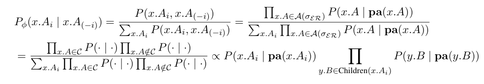
An implementation of a standard Gibbs sampler. The random walk samples the full conditional distributions of the sampling attribute in the GBN. The full conditionals are given by:
See References for more details
If True the sampler will collect samples for all event variables of the same attribute class in one block.
Number of burn in samples
Number of chains to be run
Number of samples to collect
Stores a sampled state (e.g. one value for each event variable) in the posterior.currentchain
| Parameters: | nSample – Int Count of the collected sample. |
|---|
Configuring an inference algorithm allow the algorithm to precompute as much information as possible before making inference.
In the case of Gibbs sampling, all the conditional likelihood functions, of type Likelihood, for the probabilistic attributes can be precomputed.
Inintializes a MCMC run given a Ground Bayesian Network and a set of event variables. The initial state of the markov chain is sampled using initializeVertices().
| Parameters: |
|
|---|
Creates an initial state for the markov chain by assigning a value to all sampling vertices
Dictionary of likelihood functions that are precomputed when the sampler is configured using inference.mcmc.configure()
{ key = Attribute instance : value = Likelihood of attribute }
An implementation of a Metropolis Hastings within Gibbs algorithm.
The random walk samples the full conditional distributions for normal GBNvertex instances (i.e. Gibbs sampling) and uses a Metropolis within Gibbs step to sample ReferenceVertex instances.
See References for more details
Number of burn in samples
Number of chains to be run
Number of samples to collect
Configuring an inference algorithm allow the algorithm to precompute as much information as possible before making inference.
In the case of Gibbs sampling, all the conditional likelihood functions, of type Likelihood, for the probabilistic attributes can be precomputed.
Inintializes a MCMC run given a Ground Bayesian Network and a set of event variables. The initial state of the markov chain is sampled using initializeVertices().
| Parameters: |
|
|---|
Creates an initial state for the markov chain by assigning a value to all sampling vertices
Dictionary of likelihood functions that are precomputed when the sampler is configured using inference.mcmc.configure()
{ key = Attribute instance : value = Likelihood of attribute }
Performs a MCMC sampling step, either a Gibbs step or a Metropolis Hastings. In case of GBNvertex instances we use Gibbs sampling and for ReferenceVertex instances we use a Metropolis within Gibbs step.
Note that we can exploit the conditional independence by Lazy Aggregation. When sampling all event vertices of a certain attribute, we need to perform the (potential aggregation) on the parent vertices only once (see references).
The posterior distribution results from running inference for a given query using MCMC. This module contains
The convergence diagnostics have to be called by the ProbReM project script, e.g. from outside the framework.
Plots the autocorrelation. Computed according to Probabilistic Graphical Models (p. 521).
| Parameters: |
|
|---|
Extracting the value of a node and storing it in the appropriate numpy.array, currentChain.
| Parameters: | nSample – Int Count of the collected sample, i.e. the row number |
|---|
Returns the cumulative mean of chain.
| Parameters: | chain – numpy.array |
|---|
numpy.array that is currently being used by the sampler
Dictionary mapping each event variable ID to an index used to access currentChain
Plots the Gelman Rubin convergence diagnostic, according to Probabilistic Graphical Models (p. 523).
Convergence diagnostics that plots the posterior density function (using the matplotlib histogram) mean of all the sampling variables in the currentChain. If a chainID is provided the histogram of the associated chain is plotted instead. If varIndex or gbnV is provided, only the histogram of this variable is plotted.
| Parameters: |
|
|---|
Initializes a new MCMC run. Note that onlyEvent=False, so the samples or all engine.GBN.samplingVertices are collected. But the posterior is a joint distribution over the event variables (thus the other sampling variables are already marginalized)
| Parameters: |
|
|---|
Returns the posterior mean of all the sampling variables in the currentChain. If a chainID is provided the mean of the associated chain is returned instead. If sVarInd or gbnV is provided, only the mean of this variable is returned.
The pylab.hist() method is used to compute the histogram
| Parameters: |
|
|---|---|
| Returns: | Posterior mean as numpy.array. If sVarInd or gbnV are specified, this is a single value |
Convergence diagnostics that plots the cumulative mean of all the sampling variables in the currentChain. If a chainID is provided the cumulative mean of the associated chain is plotted instead. If sVarInd is provided - e.g. the index of a sampling variable - only the cumulative mean of this variable is plotted.
| Parameters: |
|
|---|
Plots the cumulative mean of all available chains using cumulativeMean(). If the plots are to be displayed on the same figure, use the figID keyword. If the plots are to display only a specific variable, use the gbnV or varIndex keyword.
| Parameters: | kwargs – Optional arguments for cumulativeMean() |
|---|
Dictionary of vertices that we are collecting samples from (e.g. the event vertices or all sampling vertices including latent variables), set
Dicitonary containing all the samples collected during inference. It is common to run more than one chain to montitor convergence, the key/value pairs are stored
{ key = ‘chainIdentification’ : value = numpy.array }
Conditional Likelihood Functions are used to generate the full conditional sampling distributions for the Gibbs sampler implemented in inference.mcmc. A conditional likelihood function is an instance of the class CLF. Similar to a tabular CPD CPDTabular, CLF constists of a matrix, a method indexrow() that indexes a conditional variable assignment. The matrix is composed from values of the orginal CPD.
Lets say we have an attribute C with two parent attributes A, B. The CPD is given by P(C|A,B). In this case there will be two likelihood functions for attribute C:
self[A] = P(c|A,b) = L(A|c,b)
self[B] = P(c|a,B) = L(B|c,a)
We note that, as in the case of a normal CPD where the parents are ordered, the order of the conditional variabels are fixed in the likelihood function. The associated attribute is first, followed by the appropriate parents in the orignial parents. By appropriate parents we mean all parents except the parent attribute for that the likelihood function, e.g.
- For self[A], the order of the conditional parents is (c,b)
- For self[B], the order of the conditional parents is (c,a)
See the class Likelihood for more details.
| Parameters: | condValues – List of conditional values |
|---|---|
| Returns: | List of likelihood values for conditional assignment |
Calculates the log probability distribution likLogMatrix
The parentAssignment is a full assignmnet to the parent attributes to the original attribute. We remove the entry that corresponds to the likelihood attribute. Note that we actually modify this list.
| Parameters: | parentAssignment – List of values. Assignments to the parent attributes |
|---|
Returns the index for the likMatrix row that corresponds to the assignment of the conditional attributes passed in condValues
| Condvalues : | List of conditional values |
|---|---|
| Returns: | Index of likMatrix row |
Computes the number of possible conditional attribute assigments and the index multipliers needed to compute the row index of a given conditional assignment.
Likelihood matrix of type numpy.array
Dimensions of the likelihood matrix
Conditional Likelihood Functions are used to generate the full conditional sampling distributions for the Gibbs sampler implemented in mcmc.
There is an Likelihood instance for every probabilistic attribute in the PRM. It implements a dictionary which stores a conditional likelihood function of type CLF for every parent attribute of every attribute class key.
Lets say we have an attribute C with two parent attributes A, B. The CPD is given by P(C|A,B). In this case the likelihood functions of type CLF for attribute C are stored in double dictionary:
self[C][A] = P(c|A,b) = L(A|c,b)
self[C][B] = P(c|a,B) = L(B|c,a)
See CLF for more details.