In science, engineering and statistics, the field of computational sciences is continuously being developed upon and improved. One of the major barriers for the development of this field is the sheer amount of computational effort or time it takes to perform numerical calculations on potentially massive systems.
One method to drastically improve computational time is to approximate complex mathematical functions with polynomials. Once we represent any continuous function with a polynomial, compositions such as differentiation or integration become negligible, and functions such as root finding also become greatly simplified.
Furthermore, polynomials can be easily represented with a vector of coefficients. For example, the vector [1.0, 0.0, 3.0] will represent \(1 + x^{2}\).
The Chebyshev approximation
This approximation can be computed with Chebyshev polynomials. While there are several types of
Chebyshev polynomials, the first type are implemented in this project.
Chebyshev polynomials of degree n are recursively defined as:
\(T_{n}\left( x \right) = 2xT_{n - 1}\left( x \right) - T_{n - 2}(x)\), with base cases \(T_{1}\left( x \right) = x\) and \(T_{0}\left( x \right)\) = 1.
They are valid on the range of \(x\ \in \left\lbrack - 1,1
\right\rbrack.\)
The final, Chebyshev series expansion is equal to:
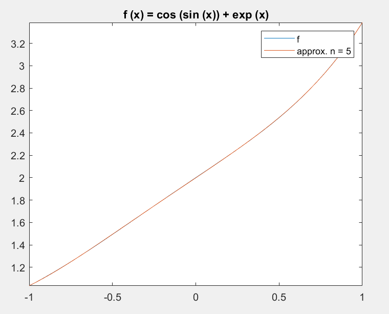
Approximating \(f\left( x \right) = \cos{(\sin{x) + e^{x}}}\)
For example, the function \(f\left( x \right) = \cos{(\sin{x) + e^{x}}}\), can be approximated by a nth order polynomial. We can see that we get a fairly good approximation of f(x) with a Chebyshev approximation of degree 5 on a range of [-1, 1].
Increasing the degree of the Chebyshev Polynomial
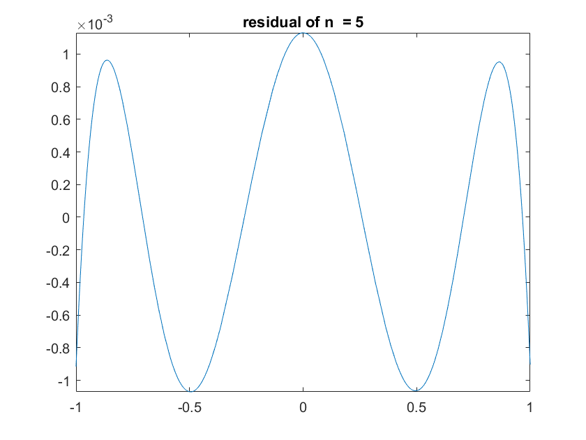
However, the goal of this library is to approximation functions to machine-level floating point precision, so that we can further manipulate the functions without having to worry too much about propagating error. This graph shows the residual between the approximation and f(x), within the range of [-1, 1] for a Chebyshev Approximation of degree 5. We can see that our error is on the order of \(10^{- 3}\).
Primary usage
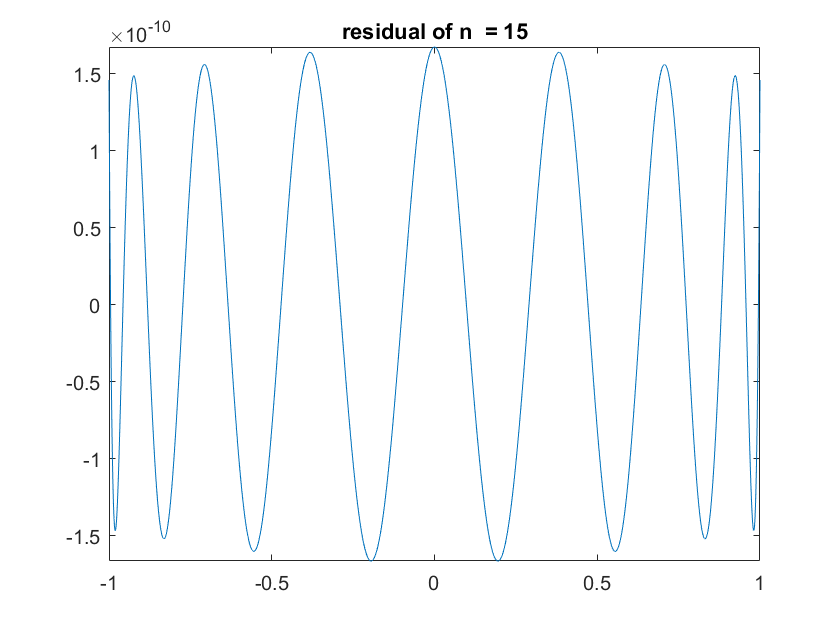
When we perform an approximation of degree 15, we can see that our results are much closer to the desired function.
This plot shows f and the approximation of the 15th order, over a domain of 1⋅10^(-9). Here, the error is on the order of \(10^{- 10}\). Eventually, if we compute a high-enough-order Chebyshev polynomial, we can sufficiently approximate any continuous function over a specified domain.
What's next?
The aim of this project is to develop a module of overloaded functions so that any function can be approximated to machine-level precision. The accelerate library, an embedded language that is conducive to quick matrix manipulations, will be used to increase the speed of the computations.
I am currently working on functions to automate the process of extending the Chebyshev polynomials, and define a robust Cheb type that can handle common arithmetic operations within the world of Chebyshev approximations.