Lesson 24 - Learning Goals

• Want area under curve between x=a and x=b

• Assume we cannot obtain an exact solution, or perhaps f(x) is unknown, and we only have data points (x_i,y_i).

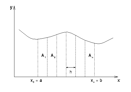
• Main idea: Break area under curve into n panels of width h: A = A_i , h = (b-a)/n
  

• How to calculate A_i ?

• Many methods of approximation

• All estimates improve with larger n, as h 0 .
  

MIDPOINT RULE

• Use rectangular panels (i.e. assume f(x) is constant and equal to y* between x_i-1 and x_i )

• Three possibilities:

• Left endpoint: y* = y_i-1 = f(x_i-1)
• Right endpoint: y* = y_i = f(x_i) = f(x_i-1 + h)
• Midpoint: y* = y_{i - ½} = f( (x_i-1 + x_i)/2 ) = f(x_i-1 + h/2)
• On average, midpoint looks like best guess
  
  

MIDPOINT RULE ALGORITHM

We wish to integrate y=f(x) from x=a to x=b using n rectangular panels of equal width.

h = (b-a) /n
x₀ = a
x_i = x_i-1 + h
A_i = h* f( (x_i-1 + x_i)/2 )
A A_i (i=1 i=n)
A h* [ f( (x_i-1 + x_i) /2 )] (i=1 i=n)

REAL FUNCTION MidPt(x0, x1, N)
! Estimate the area under F between x0 and x1
! using the Midpoint Rule with N panels.

   REAL x0, x1, x, h, Sum
   INTEGER N

   h = (x1 - x0) / N
   Sum = 0.0

   ! Add area of each panel, assuming unit width
   ! and multiplying by the true width h later.

   x = x0+h/2.0 ! Initial start is middle of first panel

   L1: DO k= 1,N
      Sum = Sum + F(x)
      x = x + h
   END DO L1

   MidPt = h*Sum

RETURN

C Version

double midpoint(double x0, double x1, int n)
{
   double h, sum;

   /* Calculate panel width h; initialize Sum. */

   h= (x1 - x0) / n;
   x0= x0 + h/2;
   sum= 0;

/* Add area of each panel, multiplying
by the true width h only once later. */

   do {
      sum= sum + f(x0);
      x0= x0 + h;
   }while(x0 x1);
   return(sum * h);
}

TRAPEZOIDAL RULE

Try taking average of the expressions for rectangular A_i, with f evaluated at left and right endpoints

A_i = [ h f(x_i-1) + h f(x_i) ]/2

A_i = h/2 [ f(x_i-1) + f(x_i) ]

Approximate A_i, as the area of trapezoid abcd.

Trapezoidal method appears to take 2 function evaluations per panel, but

A_i + A_i+1= h/2 [ f(x_i-1) + f(x_i) ] + h/2 [ f(x_i) + f(x_i+1) ]

A_i + A_i+1 = h/2 [ f(x_i-1) + 2f(x_i) + f(x_i+1) ]

For n panels, need only n+1 evaluations of f.

TRAPEZOIDAL RULE ALGORITHM

We wish to integrate y=f(x) from x=a to x=b using n trapezoidal panels of equal width.

h= (b-a)/n

x₀ = a

x_n = b

x_i = x_i-1 + h

A_i = h/2 [ f(x_i-1) + f(x_i) ]

A A_i (i=1 i=n)

A h [ ( f(x₀) + f(x_n) ) / 2 + f(x_i) ] (summing from i = 1 to n-1 )

SIMPSON'S RULE

In Trapezoidal rule, successive points (x_i, y_i) were joined with straight lines

Now, fit a parabola to 3 points (x_i-2, y_i-2), (x_i-1, y_i-1), and (x_i, y_i) for better accuracy

One panel (width 2h) now includes 3 points

h = (b-a)/n

b-a = nh

n must therefore be even

From geometry or Taylor series expansion, we find

A_i = h/3 [ f(x_i-2) + 4f(x_i-1) + f(x_i) ] , for i = 2,4,6,…,n

Once more, combine expressions for adjacent panels and simplify.

A_i + A_i+2 = h/3 [ f(x_i-2) + 4f(x_i-1) + 2f(x_i) + 4f(x_i+1) + f(x_i+2) ]

For n panels, again need only n+1 evaluations of f.

SIMPSON'S RULE ALGORITHM

We wish to integrate y=f(x) from x=a to x=b using n/2 double parabolic panels of equal width.

h = (b-a)/n
x₀= a
x_n= b
x_i= x_i-1 + h
A_i = h/3 [ f(x_i-2) + 4f(x_i-1) + f(x_i) ]
A A_i (i=1 i=n)

A h/3 [ f(x0) + f(xn) + 4 f(xi) + 2 f(xi) ]
    where first is from i=1 to n-1
    and second is from i=2 to n-2

ADAPTIVE INTEGRATION PROCEDURE

- Arbitrary precision

ADVANCED, RECURSIVE ADAPTIVE INTEGRATION TECHNIQUE

/* more sophisticated adaptive integration method

using recursion */