The Basics of Chain Coding
A line drawing is an image of line or curve segments that may be connected or disconnected. Several applications require the storage of line drawings in computer graphics, image processing, pattern recognition and even Automated Cartography in Geographic Information Systems where contours of maps have to be stored.
Freeman et al. proposed several methods called Chain Coding to represent line drawings that help efficient transmission and storage of such data. For this purpose it is required to quantize and encode the 2D figure. A uniform mesh is superimposed on the line drawing. We assume that the distance between two consecutive mesh nodes is T. A line drawing is quantized or approximated using curve points. Curve points are chosen to represent points on the line drawing by specifying mesh nodes that are close to the curve in terms of the different quantization schemes, giving different representations for each scheme. Three such quantization methods are described below.
Quantization Schemes
Square Quantization
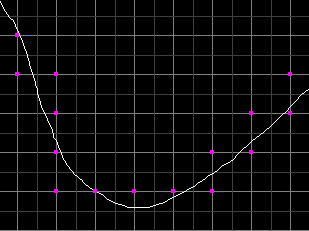
Each mesh node is taken to be the center of a square of side T as shown in the figure below. When some part of the line drawing or curve falls within the square, of a particular mesh node, that node is marked as a curve point. In the example of the curve given in the figure, this quantization scheme gives rise to the pattern with curve points shown in magenta.
Circular Quantization
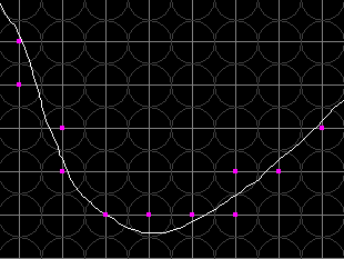
The same idea as above is applied in this quantization scheme except that each mesh node is considered to be the center of a cricle of radius T/2 as shown in the figure below. When some part of the line drawing falls within the circle, of which a mesh node is the center, that node is considered a curve point. This method gives rise to the sequence of curve points shown again in magenta in the figure below.
Grid-Intersect Quantization
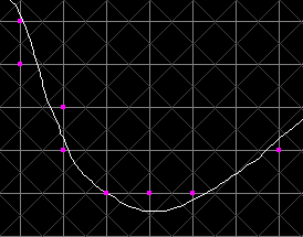
In this scheme curve points are selected according to where the curve intersects the mesh lines between adjacent nodes. Each place the line drawing intersects the mesh, the mesh nodes associated with the mesh line are considered. The node which is closer to the intersection is selected as a curve point. When there is more than one intersection point around the mesh node, only one curve point is chosen. The sequence of magenta dots arises from this process as shown in the figure below.
The approximation of a line drawing using the sequence of curve points found using any of the three quantization schemes described above can be coded using at most 8 bits per line segment. This is because for any curve point the next curve point in the sequence can be in at most eight directions as shown in the figure below.
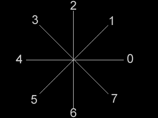
Each line segment in the approximation is given a code according to the eight directions the segment can take, giving rise to a chain code representation for each line drawing. Each of the three quantization schemes desribed yield the chain codes shown in the next figure.
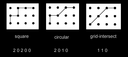
The different quantization schemes often yield very different chain codes for the same line drawing. One of the factors in which the schemes differ is the number of diagonal line segments they contain. It can be readily seen that the square quantization does not give any diagonal segments (assuming that the line drawing never passes through the intersection of two mesh lines), whereas they do occur in circular and grid-intersect quantizations. According to Freeman, diagonal elements should occur half the time for random configurations for a good or close approximation.
Minkowski Metric Quantization
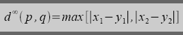
The k-Minkowski metric between two points p=(x1,y1) and q=(x2,y2) can be given as
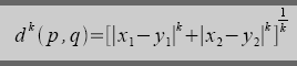
where k >= 1.
For k=2, this becomes,
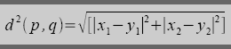
which is the Euclidean distance between the two points.
For k=∞, this becomes
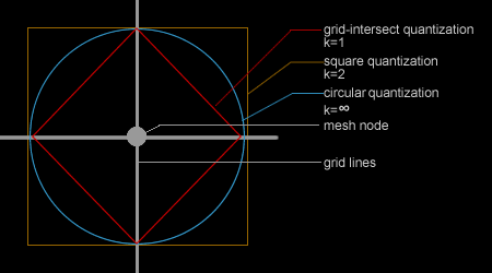
The figure below shows the locus of points around a mesh node by taking dk (p,q)= for k=1,2 and ∞. For k=∞, the locus is a square of side T. For k=2, it is a circle of radius and for k=1, it is a rhombus of diagonal T and side for k=1,2 and ∞. For k=∞, the locus is a square of side T. For k=2, it is a circle of radius and for k=1, it is a rhombus of diagonal T and side  . .
If L denotes the set of points in the line drawing, then we can give a more formal
definition of a curve point using the Minkowski metric.
Definition: For a line drawing L and a mesh gap T, a mesh node is a curve point,
according to the k-Minkowski metric quantization, if and only if the distance from the
node to the closest point in the set L is less than .
If k=∞, the quantization scheme becomes the square quantization and for k=2, it becomes
the circular quantization scheme. For k=1, a new quantization scheme arises called the
rhombic quantization. Convex quantizations can be referred to as all schemes where the region checked around the mesh node is convex.
Go to the Freeman coding demo applet | back to the Freeman Coding main page
|