Modelling and Simulation of a
Pump Control System
Sadaf Mustafiz
Miriam Zia
COMP 522
Project Report
School of Computer Science
McGill University, Montréal
December 22, 2004
Contents
2.1 Fault Tolerance Mechanisms
3. Case
Study: Pump Control System
3.2 Requirements Specification
4.3 Model of the Original System
4.4 Model of the Fault-Tolerant System
1.
Introduction
The introduction of fault tolerance design in the software development
process is an emerging area of active research. For our project, we are interested
in modelling and simulating the behaviour of a real-time system used in a mine
drainage environment, and observing how fault tolerance techniques can improve
or change some performance metrics. In particular, we would like to analyze the
dependability properties of the system which include the evaluation criteria
reliability and safety.
1.1
Project Description
The application chosen is a standard in real-time systems literature:
the pump control system (PCS). For example, Burns and Lister used PCS as a case
study to discuss the TARDIS project (Timely and Reliable Distributed Systems).
Our goals for the project are as follows:
·
to create a model for a real-time system based on the functional
properties
·
to improve the model based on non-functional properties and to integrate
fault-tolerant means into it.
·
to implement the models using PythonDEVS for simulation
·
to observe the improvement in the dependability metrics of the system
introduced by fault-tolerance
1.2
Timeline
|
Project team |
October 12, 2004 |
|
Project proposal |
October 20,
2004 |
|
Prototype 1 (non FT model) |
November 5,
2004 |
|
Final presentation in class |
December 3,
2004 |
|
Post presentation and
sources on website |
December 22,
2004 |
2.
Fault-tolerant Systems
Systems are developed to
satisfy a set of requirements that meet a need. A requirement that is important
in some systems is that they be highly dependable. Fault tolerance is a means of achieving dependability. Fault-tolerant systems aim to continue
delivery of services despite the presence of hardware or software faults in the
system.
There are three levels at
which fault tolerance can be applied. Traditionally, fault tolerance has been
used to compensate for faults in computing resources (hardware). By managing
extra hardware resources, the computer subsystem increases its ability to
continue operation. Hardware fault
tolerance measures include redundant communications, replicated
processors, additional memory, and redundant power/energy supplies. Hardware
fault tolerance was particularly important in the early days of computing, when
the time between machine failures was measured in minutes [1].
A second level of fault
tolerance recognizes that a fault tolerant hardware platform does not, in
itself, guarantee high availability to the system user. It is still important
to structure the computer software to compensate for faults such as changes in
program or data structures due to transients or design errors. This is software fault tolerance.
Mechanisms such as checkpoint/restart, recovery blocks and multiple-version
programs are often used at this level [1].
At a third level, the
computer subsystem may provide functions that compensate for failures in other
system facilities that are not computer-based. This is system fault tolerance. For example, software can detect and
compensate for failures in sensors. Measures at this level are usually
application-specific [1].
2.1
Fault Tolerance Mechanisms
 Error detection. This step involves identification of errors in the
system and uses forms of active redundancy for this purpose.
Error detection. This step involves identification of errors in the
system and uses forms of active redundancy for this purpose.
System
Recovery. Compensation, a form of system
recovery, involves the use of redundancy to mask an error by only selecting an
acceptable result based on some algorithm, thus making it possible to transform
to an error-free state. Modular redundancy along with majority voting is a
common technique to achieve compensation.
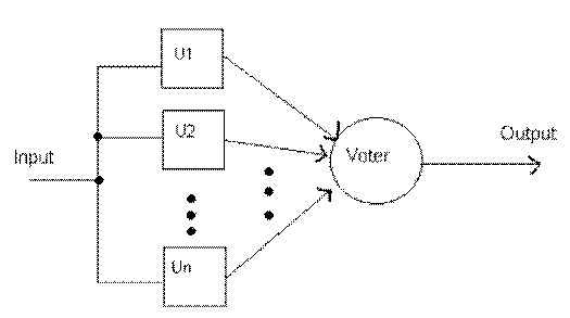
N-Modular Redundancy. This is a
scheme for forward error recovery. N redundant units (U1… Un) are
used, instead of one, and a voting scheme is used on their output. There are
many types of voters which can be used. More interestingly, the ones we use for
this implementation are the majority
voter, which given n results will output the one which reoccurs
the most, and the “maximum”
voter , which outputs the highest value from amongst the n
results received.
Figure 1.
NMR
redundancy and voting
3.
Case Study: Pump Control System
3.1
TARDIS
The Timely and Reliable
Distributed Information Systems (TARDIS) project was initiated jointly by Prof.
Alan Burns of University of York (York) and A. M. Lister of University of
Queensland (Australia) in 1990. The TARDIS framework was targeted towards
avionics, process control, military, and safety critical applications. It was
developed with the intention of creating a framework which considered
non-functional requirements and implementation constraints from the early
stages of software development.
3.2
Requirements Specification
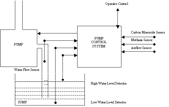
The basic task of
the system is to pump the water that accumulates at the bottom of the shaft to
the surface. Figure
2 illustrates the pump control system.
3.2.1
 Functional
Requirements
Functional
Requirements
·
Pump operation. The pump is switched on when
the water level is below the high-water level and the methane level is below
critical. In addition to automatic operation, the operator and the supervisor are
allowed to switch the pump on and off based on some conditions. The operator is
only allowed to switch on the pump when the water level is above the low-water
level, and the methane level is below critical. The supervisor however can
switch it on only based on the methane level, which has to be below critical.
The pump is switched off automatically when the water level goes below the
low-water level or when the methane level reaches the critical level. The
supervisor is allowed to switch it off only when the water level is below the
high-water level.
·
Pump monitoring. Every operation on the pump
and its state alterations are logged.
·
Environment monitoring. The environment sensors for
methane, carbon monoxide gas, and airflow need to be constantly monitored and
logged. The critical levels of these sensor values may lead to the pump being
shutdown or to alarms being raised.
Operator information. The operator
should receive information about all critical readings of sensors.
During the modelling phase, our project will abstract away from the
following:
·
Pump and environment monitoring: the logging of
the readings from the environment sensors and the pump operations will not
modelled.
·
Operator and Supervisor: these will be replaced by a
passive human controller in our model.
3.2.2
Non-functional Requirements
Burns and Lister describe
three non-functional requirements in their paper: timing, security and
dependability. For the scope of this project, we focus on the latter.
For PCS, the dependability
requirements ensure that the system is reliable and safe.
Reliability
in the pump system is measured by the number of shifts
that can be allowed to be lost if the pump does not operate when it should be.
In this case, a system can be said to be reliable if it loses at most 1 shift
in 100. Also, even on pump failure, a water accretion period of one hour is
allowed before a shift is defined as lost.
Safety
of the pump system is related to the probability that an explosion can occur if
the pump is operated when the methane level is above critical. In this case,
the probability is assumed to be less than 10-7 during the lifetime of the
system.
3.3
System Architecture
3.3.1
Logical Architecture
The logical architecture considers
the functional requirements of the system, and in this case also the security
requirement. Hence, for this system, the functional requirements can be mapped
to four classes: pump subsystem, data logger (introduced due to pump
monitoring), environment subsystem, and operator.
As mentioned previously, our
project will not look into data logging issues, and will replace the supervisor
and operator entities by a passive human controller who receives alarms but 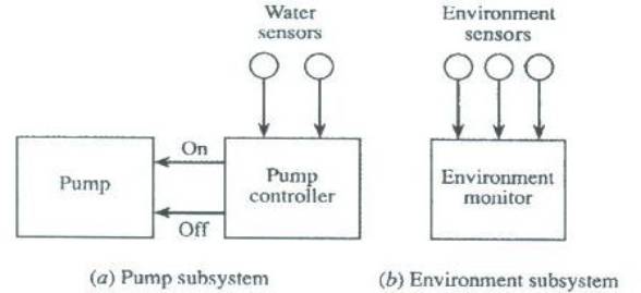 does not respond
to them.
does not respond
to them.
Figure 3.
Logical architecture of the pump control system
Figure 4.
Logical architecture refinements
3.4
Failure Scenarios
At the subsystems level,
safety of the system can be threatened due to the failures mentioned below.
- The environment subsystem sends an incorrect methane value to the
pump subsystem.
- The environment subsystem fails to generate an alarm when the
methane level goes above critical.
- The communication subsystem does not notify the pump subsystem
about the alarm.
- The pump subsystem fails to switch off the pump after receiving the
alarm.
From the above, it can be
deduced that safety of the system is dependent on the environment subsystem,
the pump subsystem, and the communication medium between them. Two types of
failures can affect safety: fail-silent and fail-noisy.
The first step would be to
create fault containment areas. The task of raising an alarm can be avoided, if
the pump subsystem can be assigned an additional operation of checking the
methane level continuously. This way the pump can switch itself off when it
receives no response from the environment subsystem. This does not increase the
design complexity. The system is now only affected by failures in a fail-noisy
manner. In addition, time-stamping may be used when sending methane readings to
enable the pump subsystem to realize when it’s getting old readings and act
accordingly.
In the case of reliability,
to prevent loss of shift, the pump should be repaired before the water
accretion period passes.
Since sensors only fail in a
fail-noisy manner, replication of the sensors is required to tolerate hardware
failure. Three sets of sensors can be used along with N-modular redundancy
(NMR) technique (discussed in Section 2.1) for detecting and tolerating faults. In a similar
way, the other components in the system can be analyzed and measures taken to
achieve dependability.
Our focus in this project is to apply fault tolerance techniques in order to solve the first failure scenario. We will implement replication using the NMR technique to produce the non-faulty system.
4.
Modelling of the System
4.1
Modelling Formalism
As the states in PCS change only in accordance
to external events, the appropriate choice of a modelling formalism is the
Discrete EVent System
specification. In addition, PCS is composed of many different interacting
subsystems, and DEVS, being highly modularized, allows for a clean model of
such a system.
4.2
Outline of the Solution
We follow an iterative
development process, comprising of the stages analysis, design, code, and
testing.
We start by designing the
real-world behaviour of PCS. Each subsystem (pump, environment, communication)
is modelled as an atomic or coupled DEVS. After modelling the functional
requirements, we need to model a fault injection mechanism. The fault injector
would alter the normal behaviour of the system on a periodic basis in order to
make a subsystem fail. For example, a fault in the methane sensor would
generate faulty (noisy) methane readings of the environment, which would be
propagated to the environment monitor, and through the communication subsystem
to the pump controller. This wrong methane reading could possibly force the
pump to shut off when it is not supposed to, or it might fail to cause a
critical alarm to be raised. The simulation results should show how the
performance varies over time in the absence and presence of faults.
Next, the model is adapted to integrate fault
tolerance techniques. Replication of sensors with maximum voting is one
possibility. For example, even if one of the methane sensors fails (caused by
the fault injector), an event is still passed on to the subsystem based on the
state of the other sensors. With the same fault injection technique, we
simulate the model to see how it behaves with FT means, as in, how the
performance changes.
The system behaviour to be
modelled is discrete event-based, it will thus be suitable to use the DEVS
(Discrete Event System Specification) formalism.
4.3
Model of the Original System
DEVS
model of the original system
4.3.1
Methane Sensor
States: This sensor may
either be READING the level of methane in the environment or IDLE between
readings. A reading is generated every 2 seconds.
Output: Upon
transitioning from READING to IDLE, the sensor outputs the level of methane in
the environment at that time. Faults will be injected internally in order to
have the sensor output an accurate reading ninety percent of the time, and a
false reading 10 percent of the time.
A methane reading is a
positive integer between 0 and 10, and is non-critical below 7.
4.3.2
Carbon Monoxide Sensor
States: This sensor may
either be READING the level of carbon monoxide in the environment or IDLE
between readings. A reading is generated every 6 seconds.
Output: Upon
transitioning from READING to IDLE, the sensor outputs the level of carbon
monoxide in the environment at that time. Faults will be injected internally in
order to have the sensor output an accurate reading 91 percent of the time, and
a false reading 9 percent of the time.
A carbon monoxide reading is
a positive integer between 0 and 10, and is non-critical below 5.
4.3.3
Airflow Sensor
States: This sensor may
either be READING the airflow in the environment or IDLE between readings. A
reading is generated every 5 seconds.
Output: Upon
transitioning from READING to IDLE, the sensor outputs the airflow in the
environment at that time. Faults will be injected internally in order to have the
sensor output an accurate reading 88 percent of the time, and a false reading
12 percent of the time.
An airflow reading is a
positive integer between 0 and 10, and is non-critical below 3.
4.3.4
Environment monitor
States: The monitor may either be processing sensor readings
('PROCESSING'), responding to a query ('QUERYING') or doing nothing ('IDLE').
Output: Upon receiving a query, the monitor responds by sending an
acknowledgement which contains a message stating whether the last methane level
received was critical or not critical. Upon receiving readings from the
environment sensor, it outputs alarms when the readings are critical.
All messages to and from the pump controller or to the human controller
are sent through the communication DEVS.
4.3.5
Pump Controller
States:
It may either be processing a water sensor reading and sending an
operation to the pump ('PROCESSING-WATER'), processing a methane alarm
('PROCESSING-ALARM'), processing a query acknowledgement ('PROCESSING-ACK'), or
doing nothing ('IDLE').
Output: Upon receiving a water low reading, the
pump controller sends an ”off” message to the pump to make it switch off. If
the controller receives a water high reading, it turns the pump to ready mode
and sends a query to the environment monitor: the controller will only ask the
pump to turn on if the methane level is not critical. If an acknowledgement is
received stating that the methane level is high, then the controller will turn
the pump off, otherwise, it will turn it on. Similarly, when the controller
receives a methane alarm, it turns the pump off.
4.3.6
Water Sensor
States: will randomly
switch between the HIGH and LOW states.
Output: the state to
which the sensor is transitioning.
4.4
Model of the Fault-Tolerant System
DEVS model of the fault-tolerant system
In this model, each of the
environment sensors is replicated 3 times. Each of these replicated sensors
behaves in a regular fashion as described in Section 4.3, and will output either an accurate or false result.
In order for all sensors to agree on the accurate reading (rather than having
each randomly generate one as in the non fault tolerant system), levels are
generated in a separate DEVS called the actualRGenerator.
actualRGenerator DEVS. Every 1.9
seconds, this DEVS will generate an accurate reading for the environment
sensors. These readings are stored globally in the class and can be accessed
without passing through in and out ports of DEVS.
The results from a set of
replicated sensors are sent to a voter. We have two versions of the fault
tolerant system modelled. In one version, we use a maximum voter, in which the
highest value received for the replicated sensors will be the one considered as
the real one. The second version implements a majority voter in which the
dominant reading is considered as the real one.
The set of replicated sensors
and their voter are combined in a coupled DEVS, the output of which is sent to
the environment monitor. From there, the behaviour described in Section 4.3 is modelled.
4.5
Performance Metrics
We keep track of two
dependability metrics: safety of the system and reliability of the sensors.
Burns and Lister describe reliability of the pump in [3], however, the pump can only fail in a mechanical way,
and recovering for this failure only implies repairing or replacing the pump.
Therefore, this is not an interesting measure of dependability for the purpose
of our project. Hence, we have replaced the pump reliability by that of the
methane sensor, as it is a safety critical component. This differs from the
description of the reliability requirement given in Section 3.2.2.
4.5.1
Safety of the system
We keep track of the safety
of the system throughout the simulation time by assuming the following:
- Whenever a methane sensor outputs the accurate environment reading,
the safety of the system is met.
- If the methane sensor outputs a false reading which is inaccurately
non-critical, then the safety of the system is threatened.
- If the methane sensor outputs a false reading which is in
accordance with the accurate reading (that is it is critical when the
accurate reading is critical, and not critical when the accurate reading
is not critical), then the safety of the system is not threatened.
This recording is done inside
the MethaneSensor DEVS, and safety failures and successes are written to file.
4.5.2
Reliability of the methane sensor
We keep track of the dependability
of the methane sensor throughout simulation time by assuming the following:
- whenever the accurate reading is output, the sensor is reliable.
- whenever the false reading is output, the sensor is not reliable.
This recording is done inside
the MethaneSensor DEVS as well, and reliability failures and successes are
written to file.
5.
Simulation
5.1
Implementation
The models were implemented
using the PythonDEVS simulator [6]. To run the simulation, two other files need to be
available in the same location: DEVS.py and Simulator.py. These files can be
found in [6].
There are 3 pythonDEVS files:
PCS.py: is the implementation
of the original pump control system, without any fault tolerance applied to it.
FTPCS-maximum.py: is the fault tolerant pump
control system with replicated environment sensors (3 copies of each) and NMR
used to detect failures. The voter here receives 3 readings and outputs the
highest value as the correct one.
FTPCS-majority.py: if the fault
tolerant pump control system with replicated sensors, however, this one uses a
majority voter.
5.2
Results
Each of the above three
models was run 5 times, for a simulation time of 2000 seconds every run. For
each run, safety and reliability were logged then analyzed.
5.2.1
Safety with PCS.py
The five experimental results
were as follows:
|
Experiment
# |
Total
readings |
Failure
cases |
Failure
Probability |
|
1 |
1000 |
26 |
2.6% |
|
2 |
1000 |
25 |
2.5% |
|
3 |
1000 |
23 |
2.3% |
|
4 |
1000 |
23 |
2.3% |
|
5 |
1000 |
30 |
3.0% |
The average probability of failure
of the safety requirement was 2.54%, which is considerably high as failure may
cause loss of life. The following graph depicts the safety of the system with
regards to time (a 1 denotes that the system satisfied the safety condition, a
0 denotes otherwise).
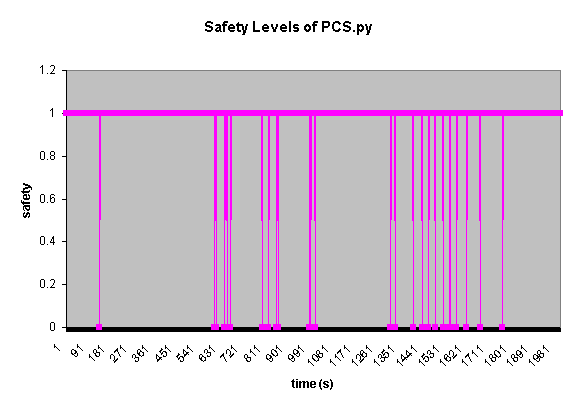
Figure 5.
Safety metric from PCS
5.2.2
Safety with
FTPCS-maximum.py
The five experimental results
were as follows:
|
Experiment
# |
Total
readings |
Failure
cases |
Failure
Probability |
|
1 |
1000 |
0 |
0% |
|
2 |
1000 |
0 |
0% |
|
3 |
1000 |
0 |
0% |
|
4 |
1000 |
0 |
0% |
|
5 |
1000 |
0 |
0% |
The average failure
probability was 0%! The following graph depicts the safety of the system with
regards to time.
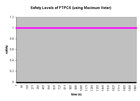
Figure 6. Safety results from FTPCS
NMR
reduces failure occurrences because it always picks the highest value to
output. It is a safe strategy at the cost of reliability, as will be shown in
Section 5.2.4.
5.2.3
Reliability with PCS.py
The five experimental results
were as follows:
|
Experiment
# |
Total
readings |
Failure
cases |
Failure
Probability |
|
1 |
1000 |
105 |
10.5% |
|
2 |
1000 |
119 |
11.9% |
|
3 |
1000 |
105 |
10.5% |
|
4 |
1000 |
97 |
9.7% |
|
5 |
1000 |
118 |
11.8% |
The average probability of the
failure of the reliability requirement was 10.88%, which is in accordance to the probability that we coded into the
methane sensor DEVS of 10% failure. The following graphs depict the reliability of
the system with regards to time (or chunks of time).
Figure 7. Reliability metric from PCS
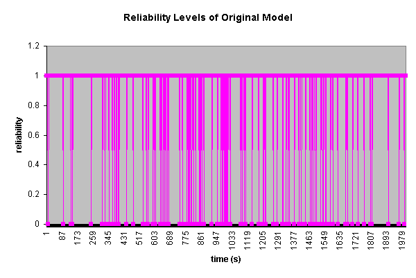
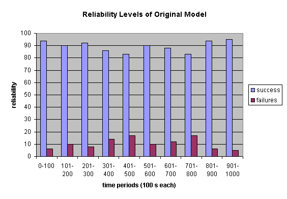
Figure 8.
Reliability metric from PCS (column form)
5.2.4
Reliability with
FTPCS-maximum.py
The five experimental results
were as follows:
|
Experiment
# |
Total
readings |
Failure
cases |
Failure
Probability |
|
1 |
1000 |
107 |
10.7% |
|
2 |
1000 |
143 |
14.3% |
|
3 |
1000 |
104 |
10.4% |
|
4 |
1000 |
111 |
11.1% |
|
5 |
1000 |
129 |
12.9% |
The sensors failed to be
reliable 11.88% of the time. The following graphs
depict the reliability of the system with regards to time (or chunks of time). This failure rate does not present much improvement
on the non fault-tolerant system. This could be explained by the fact that the
maximum voter will always pick the highest value to output, no matter if it is
the accurate one or the false one. Then we can imagine a situation where the
accurate reading is 2, but a false reading received is 8, then 8 will be voted
to be the correct reading. This is a safe situation, however, at the cost of
lowering the reliability of the sensors. Then we must devise a way in which
both safety and reliability can be met, without having large trade-offs. One
such solution would be to use a different kind of voter, namely a majority
voter.
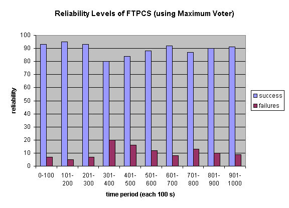
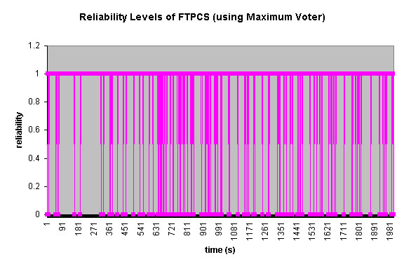
Figure 9. Reliability metric from FTPCS (maximum voting) – column form
Figure 10. Reliability metric from FTPCS (maximum voting)
5.2.5
 Reliability with FTPCS-majority.py
The five experimental results
were as follows:
|
Experiment
# |
Total
readings |
Failure
cases |
Failure
Probability |
|
1 |
1000 |
26 |
2.6% |
|
2 |
1000 |
21 |
2.1% |
|
3 |
1000 |
17 |
1.7% |
|
4 |
1000 |
31 |
3.1% |
|
5 |
1000 |
13 |
1.3% |
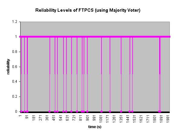
Then
the average failure rate of reliability is 2.16%! A solid improvement on the
original model and on the maximum-voting scheme. The following graph depict the reliability of the system with regards to
time.
Figure 11.
Reliability
metrics from FTPCS (majority voting)
6.
Future Work
Modelling and simulation of
the pump control system is work in progress and may be extended to model some
of the techniques mentioned by Burns and Lister for solving the other types of
failures described in Section 3.4 (failure scenarios), for example, improving
dependability of the environment monitor and the pump controller by replicating
them and using NMR for failure detection. In addition, one may experiment with
alternate FT techniques to study whether they improve PCS dependability.
However, it may also be extended to simulate other performance metrics
affecting the system, such as timeliness and security.
As mentioned earlier, the
operator and supervisor of the pump were replaced by a human controller coded
as a passive DEVS. The model could be extended to include two separate human
controllers with different access rights, and model their interaction with the
PCS.
Thirdly, a fault injector may
be modelled as a separate and external DEVS which would send events to system
components in order to provoke their failure. As it stands now, our faults are
injected within the component whose failure is desired, for example, the
methane sensor will fail-noisy 10% of the time by generating a false
environment reading.
Lastly, as a simulation is
meant to emulate real behaviour, it would be more accurate to gather real
values for the failure rates of a certain brand of environment sensors used in
practice, or a more accurate (rather than just random) function of how airflow,
methane and carbon monoxide levels vary in mining environment.
7.
Conclusion
With regards to the
simulation results, it is an obvious conclusion that both safety and
reliability are improved with the application of fault tolerance techniques,
however, depending on which type of voter to use, certain compromises are made
between safety of the system and reliability of the methane sensors. Using a majority voter optimizes the system
as both reliability and safety requirements are met and dependability of the
system is guaranteed.
It is then safe to say that
modelling formalisms used to represent system behaviour are a useful tool for
analyzing the system structure and observing where faults may occur. Simulation
results are a good indicator and measure of the non-functional requirements
that a specific system must obey.
To guarantee the design of a
fault-tolerant system, one can model “what-if” situations, that is to say every
possible way in which failures may occur, and adjust this model by adding some
fault tolerance techniques in order to improve system performance. We can go
further and inspect which amongst many fault tolerance techniques not only fix
the problem but actually optimize performance. If such a step is taken during
the design and analysis phase of any project, development cost would be reduced
(as the system would be built right the first time) while non-functional
requirements would have been addressed earlier on in the development cycle, and
simulation results would have emulated the expected behaviour of the
fault-tolerant system.
References
[2] Bolduc, J.-S.,
Vangheluwe, H., “A Modeling and Simulation Package for Classic Hierarchical
DEVS”, July 2002.
[4]
Burns, A., Lister, A.M., “A framework for building dependable systems”,
The Computer Journal, Vol. 34 No. 2, April 1991, pp. 73- 181.
http://moncs.cs.mcgill.ca/MSDL/research/projects/DEVS/.
[5] Mustafiz, S.
“Addressing Fault Tolerance in Software Development: A Comparative Study”,
M.Sc. Thesis, School of Computer Science, McGill University, June 2004.
[6] PythonDEVS website,
November 2002,
[7] Vangheluwe, H.,
“The discrete event system specification (DEVS) formalism”.