 |  |  |
The goal is to implement the CONSTANT_FLOW algorithm to find the optical flow from image sequences and furthermore implement the improved version of the algorithm.The implementation include two steps, which are Gaussian smoothing and optical flow computation.
Gaussian Smoothing
Include spatial 2D smoothing and temporal smoothing. All are implemented by a 1D Gaussian function, which has mean is 0 and variance is 1.5. Gaussian window size is 5.
Spatial 2D smoothing is done by applying 1D Gaussian row by row then column by column, which has same effects as 2D Gaussian but much more efficient than 2D Gaussian.
Temporal smoothing is done by feeding 5 consicutive image sequences. For each pixel position, do Gaussian smoothing in the order of the image sequences' time.
One point which is worth to mention is the normalization of smoothing is important. Because the sum of the 5 points of Gaussian is actually less than 1. If we choose variance a big very, the intensity will be decreased a lot after smoothing, then the image will become dark. In order to keep the image brightness as the same before, we actually need to normalize the value after Gaussian.
Here is image examples to show the effects of Gaussian smoothing.
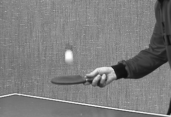
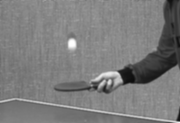
Pinpong Table(image sequence 15)
| | | |
House(image sequence 15)
 |  |  |
Optical Flow Computation
We apply a window patch on the image and move it along the image. The window size is choosen as 5 in general.For each patch, we compute the spatial gradient for each pixel and store the value in a array which is squre of window size by 2. Squre of window size is because the patch cover these many pixels. 2 is beacuse the gradient is 2 dimention. We also compute the temporal gradient and store them in a squre of window size by 1 matrix. Since the temporal has only one dimention.The spatial gradient matrix is named A and the temporal gradient matrix is named b.Once we have these two matrix, the optical flow can be computed by:
This is just the matix multiplication. There is no more to say.
For each patch, we compute a v flow. We plot the whole optical flow once we move the patch to the end of the image.
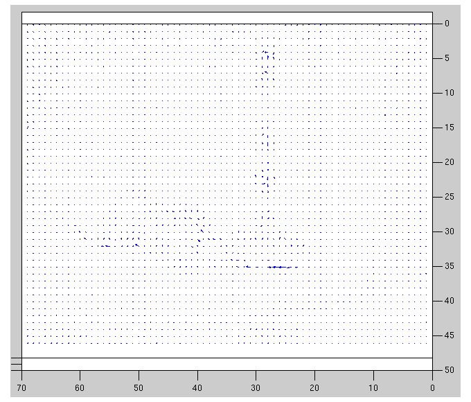
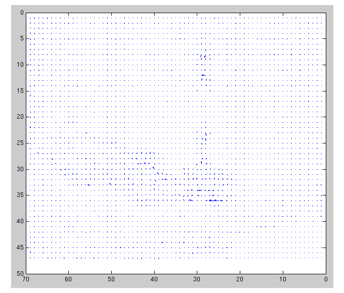
Here are two examples to show the result.
Pinpong Table
 |
 |
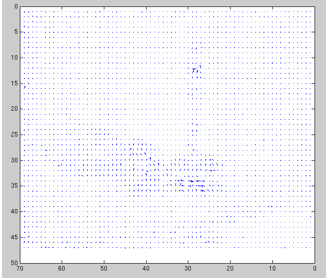 |
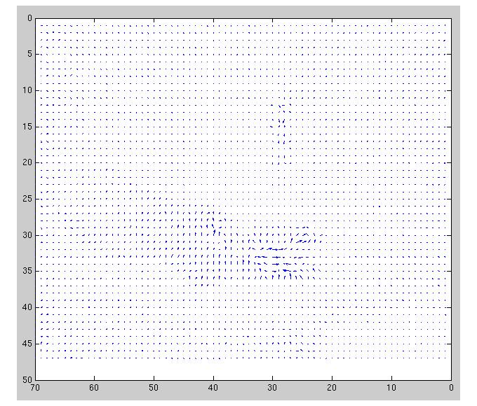 |
House
 |
 |
 |
 |
The Improved Version
It is computed by:
where the W is squre of window size by squre of windoe size. The value of the matrix is the projected 2D Gaussian. It basically functions as a mask, i.e. give the pixels which are farther away from the center of the window less weight, since they are farther away, so should weight less, and vice versa for those around center's pixels.
Unfortunately, the supposed big helper W matrix works like a killer for both house and table image. After applied the W matrix, the optical flow almost plot nothing except few arrow. For the table sequence, this probably can be explained as a good sign, e.g. only the significantly moved ball motion was show, and all the rest are wiped away by W. However, this doesn't work for the house image. Because the tree is a rigid object, it should move together.However, we can't see this from the house sequence.
The results for the improved version are shown below:
Pinpang Table
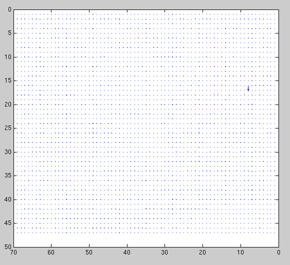 |
House
 |
We can see both flow image only show one arrow to indicate the move direction. We may say it's good, since the motion is concentratedly magnified by the unique arrow. We might also say it's bad, since the motion of the objects doesn't show at all.