308-360 Tutorial #8
1. Apply both TSP heuristics, the 2-approximation algorithm, the spanning
tree bound, the nearest neighbor bound, and the 1-tree bound to the following
distance matrix. How close to optimum is the best tour?
This problem and its 2-approximation algorithm are found on page
969 of CLR.
Heuristic: A rule of thumb, a simple rule or approach that will
help to find a good solution, though not provably an optimal solution. For
instance, a heuristic that you probably already use is that when finding a
vertex cover, it makes sense to choose vertices of maximal degree.
Lower Bound: A lower bound k of a problem
states that no valid solution to that problem can have a better
score/value than k. Note that
an algorithm to find a lower bound is not an algorithm to find the
nearest to optimal solution. It provides
information about the set of possible solutions.
2. Give a linear programming formulation for Independent Set.
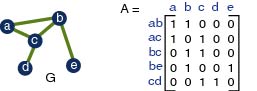
The A Matrix
The A matrix represents the input graph G. A is an m x n matrix
such that A(j,i) = 1 if vertex i is an endpoint of edge j and 0
otherwise.
The X Vector
The X vector is the variable vector representing the members of
the maximal independent set of G. Since each X entry corresponds
to one vertex and there are n vertices, there are n X entries. So
X is an n-vector. If X(i) = 1 then vertex i is a member
of the independent set. If X(i) = 0, then vertex i is not a member of the
independent set.
The Corresponding Maximal Independent Set
The size of the independent set S is therefore the number of vertices
that are members of S. It follows that |S| = sum(X(i)) for all i in X.
The Linear Programming Objective
The linear program will maximize the object function. We want
the linear program to find the largest independent set S, so to maximize the
number of vertices that are members of S. So, the objective function to
maximize is the sum(X(i)) for all xi in X.
The Linear Programming Constraint
By definition, any two vertices in an independent set must not be adjacent.
So, if vi and vj are both in the independent set, there can not be an
edge between vi and vj. For every i,j for which (vi, vj) is an edge,
X(i) + X(j) < 2. This means that either X(i) or X(j) can be set to 1, but not
both. Which is the same as saying that since (vi,vj) is an edge, only
one of its endpoints can be a member of the independent set S.
In linear programming notation, this becomes:
sum( A(j,i)X(i) ) < 2, for all j. Note that the constraint m-vector
b = 2.
The Linear Programming Solution
The linear program will find the X vector that satisfies these constraints
and provides the maximal value to the objective function.
Example (use the A matrix in the figure above)
Invalid X = [ 1 1 0 0 0 ]:
The previous X vector is invalid because both a and b cannot be
in the independent set, as they are adjacent vertices in G. Note that
in class you wrote these vectors vertically, but because of html, I'm not.
The constraint specified above therefore would not hold because at
j = 1, sum( A(j,i)X(i) ) = 1x1 + 1x1 + 0x0 + 0x0 + 0x0 = 2.
Solution X = [ 1 0 0 1 1 ]:
A possible solution to the X vector is X = [ 1 0 0 1 1 ]. This
corresponds to S = { a, d, e }. Verify the the contraint holds with this
X vector and that the objective function is maximized.