Time Slicing Assignment

Hans Vangheluwe

Fall Term 2001

The Tool

Implement (in Python) a modelling and simulation (experimentation) environment composed of:

• A causal block-diagram graphical model editor. Re-use a prototype block diagram editor. This editor exports Python code containing class definitions which, when imported in your simulation environment, will provide all model information. The most likely change you might like to make (if at all) to the modelling environment is in the saving of model information (possibly generate a single class definition). Other possible (but not necessary) changes: add input and output blocks to allow for hierarchical modelling. Your experimentation environment implementation should be independent of the model editor. In particular, the file simclasses.py should not be shared between modelling and experimentation environment.
• An experimentation environment with as its core, a Time Slicing simulator (pseudo code given in class) which takes a model description exported by the graphical model editor as well as ``experiment'' information such as

  • model initial conditions and parameters,
  • solver parameters such as step-size and communication interval,
  • where output should go (file or plot).

  Structure the simulator so it is easily embedded in different experimentation scripts (such as optimization).

  Two prototypes of the experimentation environment must be built:

  1. With a purely textual interface. Obviously, only file output of simulation results will be possible (not plotting).
  2. With a Graphical User Interface which provides a user friendly way of accessing the methods of the text-only prototype.

  Both prototypes must allow querying of model information once a model is loaded. In particular, it must be possible to ask which are the model's variables (corresponding to names of integrator blocks) and other named blocks. This information is subsequently used to set whether these must be plotted, sent to file, both, or (by default) none of the two. Data output is generated for times communication interval apart.

  At any point in time, it must be possible to save the experimentation environment's state. A small example of state saving in the form of a Python program is MyTool. Note how this is similar to the way the block diagram modelling environment passes information to the experimentation environment.

  Simulation can only start once a model has been loaded, parameters and initial conditions have been set, and simulator parameters (such as step-size) have been given. The values used by the time-slicing simulator are determined by a sequence of settings (later overrides former):

  • Default values (e.g., variables to 0, integrator step size to 0.1, ...). It should be possible to set (and save) these global defaults in the experimentation environment.
  • Values loaded from the model (e.g., initial conditions).
  • Values given interactively in the experimenation environment.

  Before starting the actual simulation, a check must be made for ``algebraic loops'' and blocks must be sorted. This will involve building a dependency graph. Algorithms can be found in the class transparencies.

• A plotting environment to display generated trajectories. It must be possible to produce both time- and phase- plots. Time-plots trace variables in function of time, phase-plots trace variables in function of one another (often [d x/d t] in function of x). The plotting environment must be capable of displaying more than one data item (trajectory). It must be possible to mix data items generated by the simulator and data items loaded from file. You will re-use the plotting environment in future assignments, so make it re-usable and as generally applicable as possible. In particular, the plotting invironment should be as independent from the experimentation environment as possible (and separately tested). The plotting environment will re-use the code from Chapter 11 of Grayson's ``Python and Tkinter'' book. As with the simulator, it must be possible to save the plotting environment's state.

The design and implementation of your tool must be documented. This is an important part of the deliverable. Use UML notation for your design.

Your tool must be thoroughly tested. Though you may include a test suite of your own making, you are strongly advised to use the PyUnit unit testing framework for Python. A short overview of PyUnit is found in the Python Library Reference.

The ``Circle Test''

Test your time-slicing simulator by means of the equation [(d² x)/(d t²)]=-x. When x and [d x/d t] are plotted in function of one another (a phase plot), a circle should result.

1. Re-write the equation in the form of a set of first order equations.
2. Draw the corresponding block-diagram in the graphical editor.
3. Run the simulation and plot the data in time and phase plots.
4. Do the above for a ``good'' (sufficiently small) integrator step-size as well as for a ``bad'' (large) step-size (which should not result in a circle plot). Explain. The ``good'' step-size will give you an idea of what step-size to use for the rest of the assignment. Explain why it should be smaller than the value you used for the circle test.

Mass-spring: simulation and calibration

The above mechanical system consists of a mass m which glides without friction over a surface. The mass is connected to a rigid wall by means of an ``ideal'' spring. In the absence of external forces, the system is in ``rest'' state and the distance of the centre of gravity of the mass object to the wall is RestLength. At any instant in time, the position (distance from the wall) of the mass is x.

An experiment has been carried out whereby the mass m was measured as well as the RestLength of the spring. m = 0.23 kg, RestLength = 0.2 m. To determine the spring constant K[kg/s²] of the ideal spring, the spring is extended to bring the mass at initial position x(t=0) with initial velocity v(t=0). x(t=0) = 0.3 m, v(t=0) = 0 m/s. (note: in many cases, in a simulation, one may have to set x(t=0) and/or v(t=0) to a small, non-zero value to avoid the simulator providing a trivial (zero) solution to the system equations).

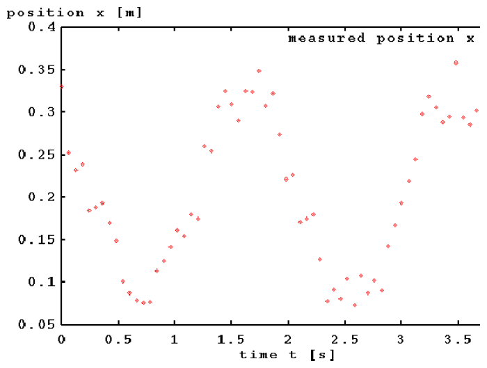
This experiment whereby the mass is released and observed during the time interval [0,4[ yields the following measurement data x_measured in function of time.

Note: this plot was produced in gnuplot from the x_measured data file (after removal of the first line) with the following commands:

 set xlabel "time t [s]"
 set ylabel "position x [m]"
 plot "data" title 'measured position x'

When you want a smooth curve rather than points, append with lines to the plot command. To plot column B of the data file in function of column A, append using A:B to the plot command.

With this ``noisy'' data, we need to ``estimate'' spring constant value K which, when used in a simulation of the dynamics of the system x(t) optimally ``fits'' the measured data. Notice how we start with parameter estimation directly and we skip the ``structure characterization phase'' in which the most appropriate mathematical model for this system is determined. This, as we have the a-priori knowledge that this is a frictionless system and the spring is ``ideal''.

Assignment:

1. Describe the mathematical equations for the dynamics of this system (given the above a-priori knowledge).
2. As this will yield a higher order differential equation, rewrite this as a set of first order differential equations.
3. Represent this set of differential equations as a causal block diagram in your block diagram modelling environment.
4. Use this in your time-slicing simulator.
5. Run multiple simulations, varying (with a small enough step-size) K value in [1, 10].
6. Check which of the K values gives the ``best fit''. Fit is defined in the ``sum of squared errors'' sense. Hereby, for each measured point in time, the difference between the measured value and the simulated value is taken and squared. The sum of all squared errors is a measure for the fit.

   Note: to give accurate results, the simulator may need a small step-size. To compare with measured data which is quite far apart, you simulator will have to implement a ``communication interval'' which allows the user to specify how often simulated values have to be output.

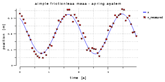
   Whether you use a very naive exhaustive search as described above or an advanced optimization algorithm (feel free to apply some of your optimization knowledge), an optimal K will result. Simulation with the ``true'' K value will yield a graph as below.

What's required

The full analysis, design (using UML notation), implementation (in Python) and simulation results should be documented and put on the web. Explicit links to code and data must be present.

You can work in groups of upto 3 people. Individual work must be indicated. All must understand and be able to explain the whole assignment (discuss your design together before implementing and do a peer review of your code).

The due date is September 26 (before midnight).