Implement (in Python) a modelling and simulation system composed of
Test your time-slicing simulator by means of the equation [(d2 x)/(d t2)] = -x. When x and [d x/d t] are plotted in function of one another (a phase plot), a circle should result.
|
|
The above mechanical system consists of a mass m which glides without friction over a surface. The mass is connected to a rigid wall by means of an ``ideal'' spring. In the absence of external forces, the system is in ``rest'' state and the distance of the centre of gravity of the mass object to the wall is RestLength. At any instant in time, the position (distance from the wall) of the mass is x.
An experiment has been carried out whereby the mass m was measured as well as the RestLength of the spring. m = 0.23 kg, RestLength = 0.2 m. To determine the spring constant K[kg/s2] of the ideal spring, the spring is extended to bring the mass at initial position x(t = 0) with initial velocity v(t = 0). x(t = 0) = 0.3 m, v(t = 0) = 0 m/s. (note: in many cases, in a simulation, one may have to set x(t=0) and/or v(t=0) to a small, non-zero value to avoid the simulator providing a trivial (zero) solution to the system equations).
This experiment whereby the mass is released and observed during the time interval [0,4[ yields the following measurement data xmeasured in function of time.
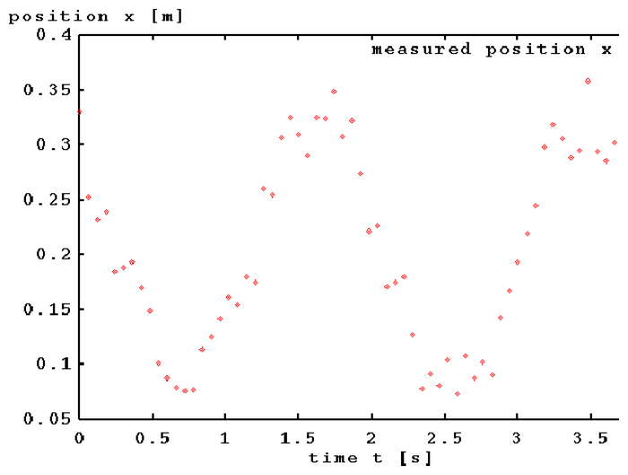 |
Note: this plot was produced in gnuplot from the xmeasured data file (after removal of the first line) with the following commands:
 set xlabel "time t [s]"</FONT>
 set ylabel "position x [m]"</FONT>
 plot "data" title 'measured position x'
When you want a smooth curve rather than points, append with lines to the plot command. To plot column B of the data file in function of column A, append using A:B to the plot command.
With this ``noisy'' data, we need to ``estimate'' spring constant value K which, when used in a simulation of the dynamics of the system x(t) optimally ``fits'' the measured data. Notice how we start with parameter estimation directly and we skip the ``structure characterization phase'' in which the most appropriate mathematical model for this system is determined. This, as we have the a-priori knowledge that this is a frictionless system and the spring is ``ideal''.
Assignment:
Note: to give accurate results, the simulator may need a small step-size. To compare with measured data which is quite far apart, you simulator will have to implement a ``communication interval'' which allows the user to specify how often simulated values have to be output.
Whether you use a very naive exhaustive search as described above or an advanced optimization algorithm (feel free to apply some of your optimization knowledge), an optimal K will result. Simulation with the ``true'' K >value will yield a graph as below.
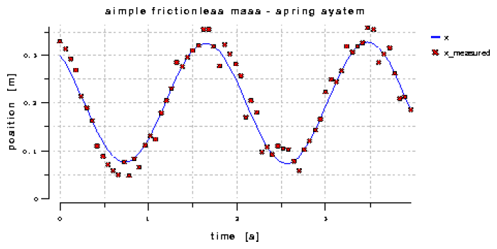 |
The full analysis, design (using UML notation), implementation (in Python) and simulation results should be documented an put on the web. Explicit links to code and data must be present.