![]() McGill University
McGill University
School
of Computer Science
COMP
765 – Spatial Representation and Mobile Robotics – Project
Local
Path Planning Using
Virtual Potential Field
By
Hani Safadi
18/April/2007
Abstract
In this report we discuss our implementation of a local path planning algorithm based on
virtual potential field described in [1]. The algorithm uses virtual forces to
avoid being trapped in a local minimum. Simulation and experiments are performed,
and compared to the results presented in the paper. They show good performance
and ability to avoid the local minimum problem in most of the cases.
Keywords
mobile robots, navigation, path planning, local path planning,
virtual force field, virtual potential field.
1.
Introduction
Autonomous navigation of a robot relies on the ability of the robot
to achieve its goal, avoiding the obstacles in the environment. In some cases
the robot has a complete knowledge of its environment, and plans its movement
based on it. But, in general, the robot only has an idea about the goal, and
should reach it using its sensors to gather information about the environment.
Hierarchical systems
decompose the control process by function. Low-level processes provide simple
functions that are grouped together by higher-level processes in order to
provide overall vehicle control [2].
We can think of high
level processing as planning level where high level plans are generated, and
low level processing as reactive control where the robot needs to avoid the
obstacle sensed by the sensors. This is called local path planning.
Local path planning,
should be performed in real time, and it takes priority over the high level
plans. Therefore, it is some time called real time obstacle avoidance.
One of the local
path planning methods, is the potential field method [3]. It is an attractive
method because of its elegance and simplicity [1]. However, using this method
the robot can be easily fall in a local minimum. Therefore, additional efforts
are needed to avoid this situation.
This report is
organized as the following:
In section 2, we
will introduce the potential field method, showing how it can be trapped to a
local minimum. Then in section 3, we will describe the modification introduced
in the paper [1], to avoid the local minimum. In section 4 will will present
our implementation of the algorithm. Section 5 will describe the test setup and
the obtained results, comparing them to the results described in the original
paper. Finally, section 6 will conclude this report.
2.
The Potential Field Method
The idea of a potential field is taken from nature. For instance a
charged particle navigating a magnetic field, or a small ball rolling in a
hill. The idea is that depending on the strength of the field, or the slope of
the hill, the particle, or the ball can arrive to the source of the field, the
magnet, or the valley in this example.
In robotics, we can
simulate the same effect, by creating an artificial potential field that will
attract the robot to the goal.
By designing
adequate potential field, we can make the robot exhibit simple behaviors.
For instance, lets
assume that there is no obstacle in the environment, and that the robot should
seek this goal. To do that in conventional planning, one should calculate the
relative position of the robot to the goal, and then apply the suitable forces
that will drive the robot to the goal.
In potential
field approach, we simple create an
attractive filed going inside the goal. The potential field is defined across
the entire free space, and in each time step, we calculate the potential filed
at the robot position, and then calculate the induced force by this field. The
robot then should move according to this force.
This figure
illustrates this concept [4]:

We can
also define another behavior, that allows the robot to avoid obstacles. We
simply make each obstacle generate a repulsive field around it. If the robot
approaches the obstacle, a repulsive force will act on it, pushing it away from
the obstacle.

[4]
The two behaviors,
seeking and avoiding, can be combined by combining the two potential fields,
the robot then can follow the force induced by the new filed to reach the goal
while avoiding the obstacle:
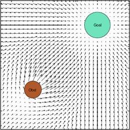
[4]
In
mathematical terms, the overall potential field is:
U(q)
= Ugoal(q) + ∑Uobstacles(q)
and the
induced force is:
F =
-U(q) = ( U / x, U /y)
Robot
motion can be derived by taking small steps driven by the local force [2].
Many
potential field functions are studied in the literature. Typically Ugoal
is defined as a parabolic attractor [2]:
Ugoal
= dist(q, goal)2
where dist is the
Euclidean distance between the state q and the goal.
Uobstacles
is modeled as a potential barrier that rises to infinity when the robot
approaches the obstacle [2]:
Uobstacles
= dist(q, obstacle)-1
where dist is the
Euclidean distance between the robot in state q and the closest point on the
obstacle. The repulsive force is computed with respect to either the nearest
obstacle or summed over all the obstacles in the environment.
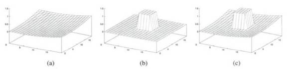
(a)
attractive field, (b) repulsive field, (c) the sum
In this
work, a more sophisticate repulsive force will be used:
Uobstacles
= (1/dist(q, obstacle) – 1/p)2
dist(q, goal)2 if dist(q, obstacle) p
0 if
dist(q, obstacle) > p
where p
is a positive constant denoting the distance of influence of the obstacle.
Potential field
method was developed as an online collision avoidance approach, applicable when
the robot does not have a prior model of the obstacle, but senses then during
motion execution [1]. And it is obvious that its reliance on local information
can trap it in a local minimum.
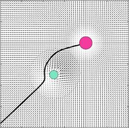
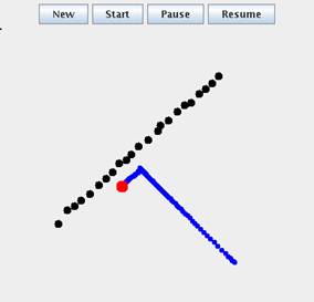
An example of that
is a U shape trap, where the robot will be attracted toward the trap, but will
never be able to reach the goal [2]:

Another example is
when the robot faces a long wall. The repulsive forces will not allow the robot
to reach the sides of the wall, and hence, it will not reach the goal.
3.
Avoiding the Local Minimum
Several methods has be suggested to deal with the local minimum phenomenon in potential filed m. One idea is to avoid the local minimum by incorporating the potential field with the high-level planner, so that the robot can use the information derived from its sensor, but still plan globally [2].
Another set of
approaches are to allow the robot to go into local minimum state, but then try
to fix this situation by:
l
Backtracking
from the local Minimum and then using another strategy to avoid the local
minimum.
l
Doing
some random movements, with the hope that these movements will help escaping
the local minimum.
l
Using
a procedural planner, such as wall following, or using one of the bug
algorithms to avoid the obstacle where the local Minimum is.
l
Using
more complex potential fields that are guaranteed to be local minimum free,
like harmonic potential fields [2].
l
Changing
the potential field properties of the position of the local minimum. So that if
the robot gets repelled from it gradually.
All these approaches
rely on the fact that the robot can discover that it is trapped, which is also
an ill-defined problem.
The method used in
this work, is similar to the last point, where the properties of the potential
fields are changed.
When the robot
senses that it is trapped, a new force called virtual free space force, (or
virtual force simply), will be applied to it.
The virtual force is
proportional to the amount of free space around the robot, and it helps pulling
the robot outside of the local minimum area. After the virtual force is
applied, the robot will be dragged outside of the local minimum and it will
begin moving again using the potential field planner. However, it is now
unlikely that it will be trapped again to the same local minimum.
More formally, the
virtual force Ff is proportional to the free space around the robot. It is
calculated by:
Ff = Fcf (cos(θ) ex
+ sin(θ)ey) [1]
where
θ is robot to free space orientation and Fcf
is
force constant
Unfortunately, the paper does not
discuss in detail what robot to free space . orientation means, nor does it
include any figure explaining ex, and
ey. However, it can be inferred that will be toward the free space around the
robot, in an opposite direction of the
obstacle. Its two components on x and y can be described by cos(θ) ex and sin(θ)ey
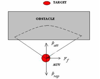
The total force will
be the sum of the attractive force (derived from the goal potential field), the
repulsive force (derived from the obstacle fields), and the virtual force:
F = Fatt + Frep
+ Ff
Finally, to detect that
the robot is trapped, we use a position estimator to estimate the current
position of the robot (open-loop). If the current position does not change for
a considerable amount of time (a predefined threshold), the virtual force is
generated to pull out the robot from the local minimum.
Note that, the robot
speed is decreased once it approaches an obstacle, (due to the repulsive
force). Therefore, the robot cannot stay in a non-local minimum place for a
long time, unless if this is planned by the high-level planner.
4.
Implementation
An implementation of the potential field algorithm, and the potential
field with virtual force algorithm is developed using the Java programming
language, we will outline it here. The full code is in the appendix with this report.
One advantage of t
he potential field method is that it is easy to implement.
We need a
representation for the robot, the obstacles, and the world.
Then at each time
step, the potential field is evaluated at the position of the robot, and the
robot is moved using the force induced by the potential field.
The
obstacle is simply a particle that has a position, a size, and a charge, in the
implementation it also provides simple methods to report the distance from the
robot.
09 double diam;
10 double mass;
11 Point p;
12 double charge;
13 public Obstacle(Point p, double charge, double diam) {
...
18 public Obstacle(Point p) {
...
24 public double distanceSq(Robot r) {
...
28 public double distance(Robot r) {
...
The robot has a
position, size, and the ability to sense the environment using methods that
simulate approximately the sonar sensor.
007 double x, y;
008 double vx, vy;
009 double dt;
010 double m;
011 double fMax;
012 ArrayList obstacles;
013 public double diam;
014 Obstacle target;
015 boolean virtualforce = false;
016 public Robot(Point p, ArrayList obstacles, double dt, double m, double fMax, double
...
028 public void updatePosition() {
...
098 boolean range(Obstacle ob, double range) {
...
106 double addNoise(double x, double mean, double stddev) {
...
The world is a set
of obstacles, and the robot. It also has the clock of the simulation where at
each time step, the robot senses the obstacle around, plan its movement using
the potential field (with or without) virtual force. And finally, perform the
action by moving its self using the potential force generated by the potential
field.
038 ArrayList obstacles = new ArrayList();
039
041 obstacles.add(new Obstacle(new Point(0, 0), +100, 3));
044 Robot r = new Robot(new Point(800, 600), obstacles, 0.1, 40, 4000, 15);
045 Thread t = new Thread();
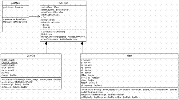
Here is the class
diagram of the project:
The interface of the
program, allows the user to create the environment adding obstacle. The running
the simulation, can controlling the addition of the virtual force.
The user can add
obstacles, turn on and off the virtual force, even when the simulation is
running. He can also pause and resume the simulation.
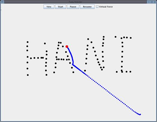
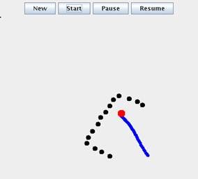
The graphical user
interface will show the robot and its path during the simulation:
5. Experiments &
Results
The potential field method with virtual force correction, is
simulated and compared to the original potential field method. The paper [1] presents two comparisons
between the two methods, proving the feasibility of the virtual force
modification.
We also performed
other experiments with our implementation, two of them were replicating the
examples shown in paper, and the others are new setups to verify the
feasibility of the modification in other situations.
The world is a 30x30
cm. The robot is treated as a particle with radius 0.7 cm, the obstacles has
radii of 1 cm. The robot uses sonar as a sensor. The simulated sonar has a
range of 5cm, and a beam width of 120 degrees [1].
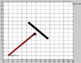
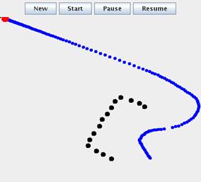
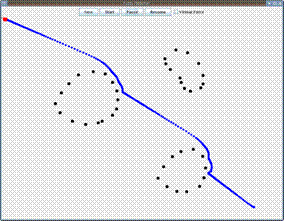
The following
experiment compares the original potential field (left) to the modified one
(right), in the U-trap example: [1]
|
|
|
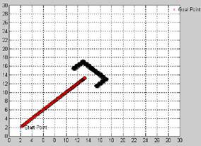
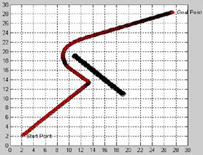
The following
experiment compares the original potential field (left) to the modified one
(right), in the wall-trap example: [1]
|
|
|
The following
experiment shows that the virtual force modification, manages to handle
navigating in complex environments: [1]
|
|
|
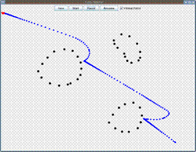
The
following experiment duplicates the U-trap situation using our implementation:
|
|
|
The
following experiment duplicates the wall-trap situation using our
implementation:
|
|
|
we notice that both
the two methods managed to avoid the wall, although the virtual force method
exhibits a more interesting behavior.
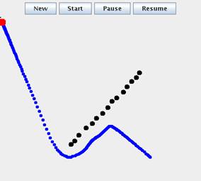
The reason might be
that the wall is not long enough, we redid the experiment with a longer wall:
|
|
|
Now the robot is
trapped, but with the addition of the virtual force it can get out of the local
minimum.
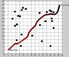
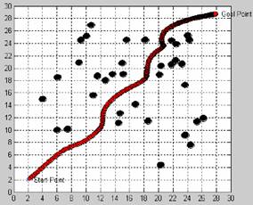
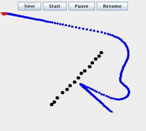
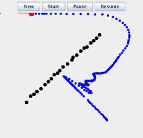
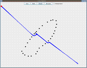
Here is
an experiment in more complex environments:
|
|
|
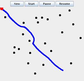
We
notice that virtual fore pulls the robots away from a set of obstacle.
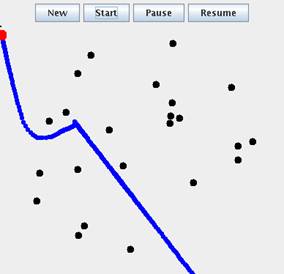
Now, we will perform
more exotic experiments, to compare the behavior both approaches (left without
virtual force, right with it):
|
|
|
|
|
|
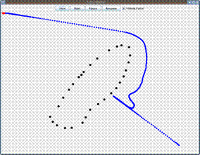
From these examples,
we notice that the virtual force robot has the tendency to stay away from
obstacles, even if there is a path near or through them. This is due to the
fact that there is no deterministic way to detect the local minimum the
heuristic used may not be accurate in several cases. This shows that although
using the virtual force will help escape from the local minimum in most of the
cases, the generated solution is not optimal, in term of path length. When no
local minimum exists the original potential field will give a better performance
than the virtual force method.
6.
Final Remarks and Conclusions
The paper [1] proposed a virtual force method for avoiding local
minimum in potential field methods. Potential field is used as basic platform
for the motion planning since it has the advantages of simplicity, real-time
computation. To get rid of the local minimum in the presence of obstacles, the
paper introduced the virtual force concept. The virtual force has been created
respectively from different condition of local minimum [1].
While this approach
manages to solve the problem in many cases, it also has several short comings:
1.
Adding
the force component seems to be a rough heuristic, if not a very ad-hoc
practice. Defining the force strength and orientation is also more as art than
a science.
2.
Adding
the force can also make the robot exhibit strange behavior, like begin
obstacle-phobic. A robot that always flees from obstacles, even if they do not
block its way completely is kind of strange.
3.
The
path generated by the virtual force method is not optimal, in fact it can be
far from optimal in certain case, due to oscillation between obstacles and free
space. (see the wall example)
4.
Adding
the virtual force, relies on the ability of the robot to detect that it is in a
local minimum. This is in practice very difficult, since the robot will not
land exactly on the local minimum [2]. And because determining the minimum also
relies on heuristics that also degrades the robustness of the method.
5.
The
local minimum is not guaranteed to be avoided, this might happen if the force
strength and orientation is not suitable with the environment dimensions.
6.
Adding
this force may also make situation that are solvable by the original potential
field, unfeasible. For instance, when the path to the goal is from a small
space within obstacle.
In my opinion, using
heuristic can be beneficial sometimes, but it is not guaranteed to be optimal.
A systematic approach is more suitable to solve this on line planning problems,
because it can be analyzed formally without throwing all this kind of constants
and heuristics. For instance, if the robot uses the bug algorithm when it hits
an obstacle, then it can avoid the local minimum, and the performance will not
suffer from the problems 1,2,5,6.
7.
Acknowledgments
We would like to thank the people whom he had very interesting
discussions. Most notably, professor Gregory Dudek from McGill university
who was always keen to discuss and help
during its stage, and many other students an colleagues in COMP 765 class, at
McGill University for interesting discussions and ideas.
8.
References
- Ding Fu-guang; Jiao
Peng; Bian Xin-qian; Wang Hong-jian, AUV local path planning based on
virtual potential field, Mechatronics and Automation, 2005 IEEE
International Conference, Vol.4, Iss., 2005 Pages:1711-1716 Vol. 4
- Gregory Dudek and
Michael Jenkin,Computational principles of mobile robotics, Cambridge
University Press, Cambridge, 2000, ISBN: 0-521-56021-7.
- O. Khatib,
Real-time Obstacle Avoidance for Manipulators and Mobile Robots,
Proceedings of the IEEE International Conference on Robotics &
Automation, pp.500-505, 1985.
- Michael A.
Goodrich, Potential Fields Tutorial,
http://borg.cc.gatech.edu/ipr/files/goodrich_potential_fields.pdf
8. Appendix I, Source Code:
|
01 package virtualforcerobot; |
|
||
|
|||
|
[4] [5] [6] [7] [8] [9] [10] 001 package virtualforcerobot; |
|
||
|
|||
|
[14] [15] [16] [17] [18] [19] [20] 001 |
|||
|
[24] [25] [26] [27] [28] [29] [30] 01 package virtualforcerobot; |
|
||
|
|||