Two Simple Solution to the Problem

Two (and too) Straightforward Approaches

Here we consider two relatively simple solution for computing D^k_nOutliers.

Block Nested Loop Join Algorithm:

The nested loop algorithm is rather a brute force solution to the problem. It computes the distance from each point p to all the other points and if the distance is less than the currently recorded distance from the k-th Nearest neighbor, it adds the point in the neighborhood list of p and updates the current value of D^k(p). Finally it takes n points with the most largest D^k(p) values as the outliers. The nested loop algorithm is as follows:

Initialize D^k(p) with infinity for each point p in database

loop through each point p in database

for each point q in database such that p≠ q

if (distance(p,q) < current estimate of D^k(p) ) then

Add q to the neighborhood list of p

new estimate of D^k(p) = distance(p, currently estimated k-th NN of p)

Sort all the points according to the descending order of D^k(p)

Select the top n points in the sorted list as the outliers

However the main disadvantage of this method is the computational complexity. It has a time complexity of O( δN²) where N is the number of input points and δ is the number of dimension. For large N or δ , this complexity reduces the efficiency of the algorithm.

Index Based Join Algorithm:

Index Based Join algorithm uses Spatial Index Structure like R* Tree to store the input points. Using a spatial index structure substantially reduces the number of distance computations. Although the original implementation in [RRS00] uses an R* Tree, in practice, any spatial index structure could be used instead.

Any Spatial Index structure, in principle, represents the whole set of point using a tree like data structure. The points that are closer to each other are placed in the same subtree. The leaves of the tree are actually the Minimum Bounding Rectangle (MBR) of a number of points. For a detailed description of R* Tree, refer to [BKSS90]. For some excellent interactive applets for Spatial Tree structures, try: http://www.cs.umd.edu/~brabec/quadtree/.

Let's consider an example to get an idea about how R* Tree keeps the data points efficiently.

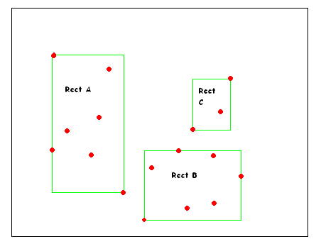
Figure 1: Some Points and their MBRs

In Figure 1, the red points are the data, and the rectangle A, B and C are the MBR for three separate subsets of points. We will not explore how the MBRs are obtain, just assume that there is an efficient way of finding the MBRs. Then, the resulting R* tree will look like Figure 2.

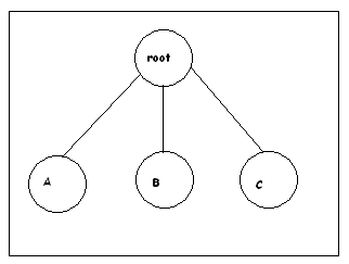
Figure 2: Corresponding R* Tree for Figure 1

Observations that make life easier:

The Index Based Join reduces the number of computation by utilizing the result of the following observation:

1. The distance of the k-th NN from any point p, D^k (p), is monotonically decreasing as we do more distance comparisons with point p.

2. We have to compute only n outliers with topmost D^k(p) values.

Both these observations are quite obvious. We start with D^k(p) value of infinity, and as we move along the loop, we update D^k(p) only if the new value is less than the old value. So, D^k(p) is always monotonically decreasing. The second observation is obvious from the definition itself.

The first observation is that, the current value of D^k (p) provides the upper bound for the actual D^k (p). Now, if the minimum distance between p and an MBR of some points exceeds the current D^k (p) value, none of the points in the MBR is to be amongst the k Nearest Neighbor of p. So, we do not need to compute distance between p and all the points in the MBR. It reduces the number of computation to a great degree. Figure 3 will present this phenomena.

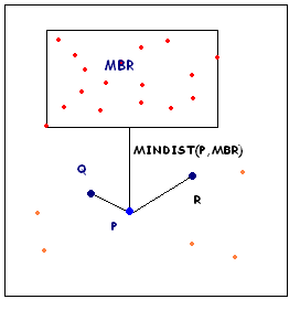Let us assume that k=2. So the distance from the 2nd nearest neighbor is considered. Assume that the current point is P. R and Q are two neighboring points which is in the neighbor list of P. The MBR of the red points is shown. Red and orange points have not been considered yet for the Nearest neighbor calculation of P.

At this moment, P knows only about two of its neighbor, Q and R. As k=2, the current D^k(p) value is Distance(P,R).

Now P finds out that MinDist(P, MBR) > current D^k(p) value. As a result, it is obvious that none of the points inside the MBR can be a candidate for 1st or 2nd nearest neighbor of P, because both Q and R are closer to P than any point in the MBR is. So, P can safely prune all the red points in the MBR from its search of neighbors. Now, only the orange points are to be searched by P.

Figure 3: Optimization using Observation 1

The second observation, along with the first, also reduces the time complexity to a considerable amount. To utilize this observation, at each step of the algorithm, the set of n points that are considered as outliers so far, are kept in a heap, such that the point with the smallest value of D^kis on the top. If the D^k (p) computed so far for a point p falls below the smallest value of D^k in the outlier heap, i.e the D^k value of the top point of the heap, there is no way can p be an outlier, because the D^k (p) value is not among the top D^k values computed so far. As it is guaranteed that p is not an outlier, further computations involving p is useless. Therefore, the Index Based Join Algorithm doesn't go any further along with that point p. Figure 4 will explain this clearly.

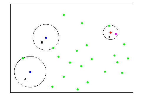Let's assume that k=1 and n=2. So, only 2 outliers are to be returned and only one nearest neighbor is to be considered in calculation.
So far, the candidate for outliers are A and B, for whom, the nearest neighbor calculation is already over. The radius of the circles centered at A and B denote the distance of respectively A and B from their respective nearest neighbors. P is the current point being considered. The nearest neighbor calculation is still going on with P. Still the magenta point has not been considered for the NN calculation of P. The current value of D^k(P) is denoted by the radius of the circle centered at P.

It is clear that current D^k(P) < D^k(A) and current D^k(P) < D^k(B).

So, P cannot be one of the 2 outliers, as both A and B will beat P in the race of being an outlier. Even though the calculation of NN of P is not fully over yet (majenta point still to be considered), we can safely discard P from being an potential outlier.

Fig 4: Optimization using Observation 2

Description of the Algorithm:

The index based algorithm is given below. The outlier heap is just a heap data structure to store the candidate for n outliers. The heap is kept sorted in the ascending order of D^k(p) values, such that the top point contains the point with smallest D^kvalue.

Initialize D^k(p) with infinity for each point p in database

Insert all points into the Spatial Tree

Initialize outlier_heap to be empty

loop through each point p in database

compute D^k(p)

If ( D^k(p) > min(D^k value for a candidate outlier in outlier_heap) )

add p to the outlier_heap and also ensure that the heap size <=n

At the end: outlier_heap will contain all the n outliers to be returned.

Seems quite simple, isn't it ? But how to compute the D^k(p) for each p ? The algorithm for computing D^k(p) is given below: Here another heap called neighbor_heap has been used. This heap keeps track of k neighbors for each point p during each iteration. Each neighbor is sorted in heap in the descending order of their distance from p.

Traverse the spatial tree based on the MINDIST between p and each node

if you reach a leaf node denoting the MBR of some points

for each point q in MBR

if ( distance ( p , q ) < min ( D^k value of a candidate outlier in outlier_heap))

Insert q into the neighbor_heap of p and also ensure that the heap size <= k

new estimate of D^k(p) = max( distance( p, any point in the neighbor_heap of p ))

if (D^k(p) <= min(D^k value for a candidate outlier in outlier_heap) )

Immediately stop calculating D^k value for p, as p will not be an outlier anyway (Ob. 1)

For each node in spatial tree

if( D^k(p) <= MINDIST ( p, MBR of the points in the node ))

Prune the whole MBR from the neighbor calculation of p (Ob. 2)

Return D^k(p)

The full pseudocode with implementation details can be found in the paper [RRS 00].

Performance:

As we can see, the D^k(p) computation algorithm uses the Observation 1 & 2 to decrease the number of comparisons to be made, and thus improves performance. The performance of this Index Based Algorithm is better than the Nested Loop based algorithm. However, still it doesn't avoid redundant comparisons to a full extent. Because, for each point in the input data set, the D^k (p) computation is initiated. The partition based algorithm described in the next page is devised to eliminate this shortcoming.

Prev: Concepts and Notations Next: Partition Based Solution

Fireworks Photo Caption